

Abstract
This study evaluates an innovative field-scale targeted sampling strategy within a regional hybrid spatial prediction model that combines machine learning and geostatistics. The framework is designed so that newly collected field observations are incorporated only through the local residual kriging step, while the regional Random Forest trend model remains unchanged, allowing field-scale predictions to be refined without full model refitting. The proposed sampling approach integrates a Normalized Difference Vegetation Index (NDVI)-based Productivity Index, a field-specific index derived from long-term satellite-based NDVI time series, with regional model-derived prediction uncertainty. The approach was evaluated on 28 test agricultural fields containing 7 to 19 in-field soil organic carbon (SOC) observations, which allowed assessment across diverse sampling configurations and levels of within-field variability. The results showed that the regional model alone provided a reasonable baseline prediction (mean root mean square error (RMSE) = 0.24% SOC) but was unable to adequately represent local spatial heterogeneity. Incorporating all available field observations produced the highest accuracy (mean RMSE = 0.17% SOC), while the proposed targeted sampling strategy achieved comparable performance (mean RMSE = 0.18% SOC) using only four strategically selected samples. In contrast, the results also showed that seemingly representative random sampling can lead to poor predictions when informative locations are missed, in some cases performing even worse than the regional model alone. In addition to conventional accuracy metrics, minimum detectable change (MDC) was used to evaluate the capability of the framework to detect meaningful SOC changes beyond prediction error, relevant for SOC monitoring and carbon farming. The results demonstrate that integrating regional models with productivity-based targeted sampling can substantially improve field-scale SOC prediction while avoiding the risks of misleading assessments associated with unfavorable sampling configurations.
Introduction
Soils represent a major global carbon reservoir, which stores substantially more carbon than the atmosphere (Lal, 2004; Schmidt et al., 2011). As a key component of terrestrial ecosystems, soil organic carbon (SOC) is fundamental to soil fertility, structure, and biological activity, while also playing a central role in climate regulation and ecosystem sustainability (Amelung et al., 2020; Batjes, 2019; Chambers et al., 2016; Minasny et al., 2017).
This recognition has driven an increasing interest in agricultural practices that enhance SOC storage, particularly carbon farming, which aims to capture and retain carbon in soils, reduce greenhouse gas emissions, and preserve existing carbon stocks (Paul et al., 2023; Sachin et al., 2026; Van Hoof, 2023). Therefore, accurate SOC information is essential for transparent carbon accounting, allowing farmers to improve soil management while ensuring that carbon credit schemes are based on verifiable outcomes (Paustian et al., 2019).
At the same time, advances in digital soil mapping (DSM), including the integration of geostatistical methods, machine learning algorithms, remote sensing data and proximal soil sensing techniques, have demonstrated great potential to produce continuous spatial SOC predictions across multiple spatial scales (Dhawale et al., 2021; Jangir et al., 2026; Khaledian & Miller, 2020; Kumar et al., 2018; Lamichhane et al., 2019; Parvizi & Fatehi, 2025; Wadoux et al., 2020, 2023).
Among the many machine learning techniques used in DSM, Random Forest (RF) has been widely recognized as a powerful prediction method due to its ability to model complex, non-linear relationships between soil properties and environmental covariates. In addition, RF is well suited for extensions that account for spatial dependence and can be effectively combined with geostatistical techniques within hybrid prediction frameworks such as Random Forest Regression Kriging (RFRK) (Hengl et al., 2018; Ho et al., 2024; Kaya et al., 2022; Sekulić et al., 2020a, 2020b; Talebi et al., 2022; Wadoux et al., 2020).
Remote sensing data, particularly vegetation indices and hyperspectral images, have become invaluable for accurate mapping and monitoring of SOC, as they provide continuous spatial and temporal information that can support and improve soil property models (Deng et al., 2025; Pouladi et al., 2023). Despite these advantages, the use of remote sensing covariates may introduce uncertainty because spectral responses are sensitive to external surface conditions, including crop residues and soil moisture, which can mask underlying soil properties (Wang et al., 2022).
The sampling strategy is widely recognized as a key factor influencing the accuracy of soil mapping models, as well-designed schemes can better capture environmental variability. Consequently, optimal sampling design has been extensively studied, particularly at regional scales (Petropoulos et al., 2025). Approaches that integrate environmental covariates and model uncertainty have proven effective in improving sampling efficiency while reducing the number of required observations. Among the most commonly used methods are conditioned Latin hypercube sampling (cLHS) (Minasny & McBratney, 2006) and Feature Space Coverage Sampling (FSCS) (Brus, 2019). Although several studies highlight the ability of cLHS to improve the representativeness of the environmental feature space (Schmidt et al., 2014; Worsham et al., 2012), others report contrasting results, indicating that the optimal strategy depends on the objectives of the study, the availability of data and the spatial scale (Ma et al., 2020; Wadoux et al., 2019). Alternative approaches have also been proposed to incorporate ancillary environmental information into sampling design. For example, Falk et al. (2011) used Local Moran’s I–based stratification, while Simbahan and Dobermann (2006) combined environmental covariates with spatial clustering and simulated annealing to optimize sampling for regression kriging. Dhawale et al. (2014) further demonstrated that proximal soil sensing data, integrated with multilayer spatially constrained clustering, can support within-field sampling design by delineating soil variability and identifying representative locations for targeted soil analysis. Beyond the choice of sampling design, the sample size remains a critical factor. Saurette et al. (2024) showed that when sample sizes are small, differences between sampling strategies (e.g., cLHS, FSCS, Simple Random Sampling (SRS)) become less pronounced. On the field scale, Žı́žala et al. (2024) emphasized that sampling efficiency is strongly dependent on the relationship between soil properties and environmental covariates, highlighting the importance of site-specific information and expert knowledge. In general, these findings suggest that effective soil sampling strategies depend not only on the choice of algorithm, but also on sample size and relevance of environmental covariates, particularly at finer spatial scales.
Among the environmental variables that may support soil sampling design, land productivity is particularly relevant because it integrates the combined effects of soil conditions, management, and crop performance (Li et al., 2025). Its importance is also reflected in Sustainable Development Goal (SDG) Indicator 15.3.1, adopted by the United Nations to monitor land condition and degradation, where land productivity is used as one of the three core sub-indicators.
Despite substantial progress in SOC mapping at regional scale, translating these approaches to the farm scale remains challenging. SOC often varies considerably within individual fields due to local soil conditions, management practices, and crop productivity patterns. A recent study by Etezadi et al. (2026) demonstrated that multi-temporal satellite imagery alone may be insufficient to describe soil variability within the field, highlighting the importance of integrating remote sensing with soil information. Previous studies have also shown that the detectability of SOC change depends strongly on sampling design, sampling density, and monitoring intervals, with detectable changes often requiring several years even under favorable conditions (Deluz et al., 2020; Gubler et al., 2019; Schrumpf et al., 2011; Smith, 2004).
Therefore, accurate SOC estimation at this scale is essential for precision agriculture, soil management, and reliable monitoring of soil carbon dynamics (Batjes et al., 2024). At the same time, farmers are increasingly seeking practical guidance to implement carbon farming practices, including clear recommendations to monitor changes in SOC over time.
Building on these challenges, this study tests the hypothesis that a small number of strategically selected field observations can substantially improve field-scale SOC prediction when combined with a regional Random Forest Regression Kriging model. Because Normalized Difference Vegetation Index (NDVI) is widely used as a proxy for land productivity dynamics (Schillaci et al., 2026), we derive an NDVI-based Productivity Index from long-term NDVI time series to characterize within-field spatial variability in crop productivity for targeted soil sampling. More specifically, we evaluate whether samples selected using NDVI-based productivity patterns together with regional model uncertainty can achieve prediction performance close to that obtained when all available field observations are included.
To test this hypothesis, we first assess the performance of the regional model when applied directly to agricultural fields without any local observations. We then evaluate how prediction accuracy changes when field observations are incorporated only through the local residual kriging step, without refitting the regional Random Forest trend model. Finally, we compare the proposed targeted sampling strategy with both the full-sample benchmark and unfavorable sampling configurations to quantify its potential benefit, as well as the loss in predictive performance associated with poorly selected sampling locations. Model performance is assessed not only using conventional point-based accuracy metrics, but also through the Structural Similarity Index (SSIM), which is used to quantify the spatial agreement among rasterized field-scale SOC prediction maps produced under different sampling scenarios.
Beyond conventional prediction accuracy, the study also evaluates the proposed framework from the perspective of soil organic carbon monitoring for carbon farming applications. In this context, prediction accuracy alone is not sufficient, as Monitoring, Reporting, and Verification (MRV) systems require a clear distinction between true SOC changes and changes that may simply reflect model uncertainty. To address this, we use the minimal detectable change (MDC) as an additional evaluation criterion, allowing us to assess whether the proposed framework can support reliable detection of meaningful SOC changes at the field scale.
Materials and methods
Case study area
The study was conducted in the Autonomous Province of Vojvodina, located in the northern part of the Republic of Serbia (Fig. 1). Vojvodina covers an area of 21,614 km2, which represents approximately 28% of the total territory of Serbia. The region is predominantly agricultural, with approximately 94.8% of the land classified as agricultural land, of which 77.8% are arable land and 6.8% are covered with forest. The dominant soil types include chernozem, covering approximately 938,881 ha (44% of the total area), semigley soils with 370,496 ha (17%), primarily associated with arable land, and humogley soils covering 348,846 ha (16%), which are more commonly found under forested areas (Djurović, 2022).

Digital elevation model (DEM) of the Autonomous Province of Vojvodina, Republic of Serbia. The inset map shows the location of Vojvodina within Southeast Europe
The Vojvodina region is relatively the most represented in both total and used agricultural land. The content of soil organic matter (SOM) in Vojvodina is strongly influenced by anthropogenic factors. According to global assessments, Vojvodina’s soils exhibit a negative balance of organic matter, suggesting ongoing degradation of soil fertility and deterioration of physical and chemical soil properties (Sekulić et al., 2010). These findings are corroborated by a study covering the period 1991 to 2013, which reported a significant decrease in SOM in various types of soils (Vasin et al., 2021). Specifically, the decline in SOC content was 15% for chernozem, 12% for semigley, and 11% for humogley soils (Vasin et al., 2021).
Data set
SOC observations
The data set includes 1196 SOC observations from topsoil, measured in 2020–2021 for the territory of Vojvodina Province, Republic of Serbia. Data was collected and prepared by the Institute of Field and Vegetable Crops from Novi Sad. The laboratory analyses were performed using Tyurin’s bichromatic titrimetric method. The working principle of this method is based on the oxidation of soil organic matter, which is carried out with \(0.4\hspace{0.25em}\mathrm{N}\hspace{0.25em}{\mathrm{K}}_{2}{\mathrm{Cr}}_{2}{\mathrm{O}}_{7}\) using an oxidoreduction indicator. It is important to note that Tyurin’s method provides lower SOC values than the widely used dry combustion method (Shamrikova et al., 2022). However, it is still used in many countries to determine SOC dynamics in studies based on historical legacy data. SOC values are reported in percent (%), i.e., grams of C per \(100\hspace{0.25em}\mathrm{g}\) of soil.
Spatially, observations are unevenly distributed over the territory of Vojvodina. An increasing density of observations can be observed from north to south as well as from east to west (Fig. 2). Generally, the dataset comprises point observations on one hand and spatially clustered observations regularly collected within fields (in-field observations) on the other. The number of observations per field varies from \(2\) to \(19\).

Spatial distribution of SOC observations across the Autonomous Province of Vojvodina (Republic of Serbia). Black crosses represent training data, while red crosses indicate test observations. The inset shows a zoomed-in view of a selected area, illustrating the local spatial arrangement of the training and test data
Environmental layers
To develop the regional prediction model, a set of 13 environmental layers was used as covariates (Fig. 3). All datasets were obtained from open-access sources. Before analysis, all layers were resampled to a common spatial resolution of 30 m, cropped to a consistent spatial extent, and reprojected to a common coordinate reference system (Universal Transverse Mercator (UTM) projection, Zone 34 N). The covariates were grouped into four categories:
-
1.
Remote sensing indices. The Normalized Difference Vegetation Index (NDVI) and Enhanced Vegetation Index (EVI) were derived from a total of 1,071 Sentinel-2 images acquired during the period 2020–2021 from the European Space Agency (ESA) data hub (Drusch et al., 2012). The dataset covers 12 tiles (scenes) with varying temporal coverage. All images (10 spectral bands) with less than 10% cloud or snow cover were processed and resampled to a spatial resolution of 10 m. Scene-level averages of NDVI and EVI were computed and subsequently mosaicked to produce continuous layers covering the entire study area.
-
2.
Soil-related covariates. Soil-related covariates, including bulk density, sand content, clay content, cation exchange capacity (CEC), and soil pH measured in water (pH_H₂O), were obtained from the Open Environmental Data Cube Europe. (Witjes et al., 2023) (https://eco-datacube.eu), with a spatial resolution of 30 m for the period 2020–2023.
-
3.
Climate-related covariates. Climate-related covariates, including precipitation and minimum, mean, and maximum air temperature, were derived from the MeteoSerbia1km dataset (Sekulić, et al., 2020a, 2020b) for the same period as the SOC observations, namely 2020–2021. The MeteoSerbia1km dataset is the first daily gridded meteorological dataset for Serbia with a spatial resolution of 1 km. The dataset includes daily, monthly, and annual summaries of meteorological variables and was generated using the Random Forest Spatial Interpolation (RFSI) methodology (Sekulić et al., 2020a, 2020b).
-
4.
Relief and topography-related covariates. A Digital Elevation Model (DEM) was obtained from the Open Environmental Data Cube Europe (Witjes et al., 2023) at a spatial resolution of 30 m.

Spatial distribution of predictor variables used for SOC modelling, arranged by covariate group. The maps include remote sensing indices (1A–1B), soil-related covariates (2A–2F), climate-related covariates (3A–3D), and relief/topography-related covariates (4A)
NDVI-based productivity index
The NDVI-based Productivity Index serves as a proxy for estimating the spatial variability of land productivity within an agricultural field and is calculated as follows. For each date, the mean NDVI value of all valid pixels within the agricultural field is calculated as:
where \({\overline{\mathrm{N}\mathrm{D}\mathrm{V}\mathrm{I}}}_{\mathrm{t}}\) is the average NDVI of the field on date \(\mathrm{t}\), and \({\mathrm{n}}_{\mathrm{t}}\) is the number of valid pixels without missing values on that date.
The relative difference between the pixel NDVI and the field mean NDVI is then calculated for each pixel and each date:
where \({\mathrm{RPI}}_{\mathrm{p},\mathrm{t}}\) is the relative productivity index of pixel \(\mathrm{p}\) on date \(\mathrm{t}\), expressed as a percentage.
The final Productivity Index is calculated as the average relative productivity of each pixel across all selected dates:
where \({\mathrm{PI}}_{\mathrm{p}}\) is the final Productivity Index for pixel \(\mathrm{p}\), and \(\mathrm{T}\) is the number of valid dates used in the calculation. Positive values indicate zones with consistently above-average productivity, while negative values indicate areas with below-average productivity relative to the field mean.
In this study, the regional SOC model was developed using NDVI and EVI covariates derived from Sentinel-2 imagery acquired during 2020–2021. In contrast, the Productivity Index was derived from a longer Sentinel-2 NDVI time series starting in 2018 to represent stable multi-season patterns of within-field productivity. Only high-quality cloud-free observations were retained to ensure the consistency and reliability of the index. The resulting dataset captures both seasonal and inter-annual variability in vegetation productivity, providing a robust representation of persistent productivity patterns within agricultural fields.
It is important to note that the Productivity Index is field-specific and cannot be directly compared across different fields, as values are normalized within each field. Nevertheless, the index provides valuable information on spatial variability within the field, enabling the identification of consistently high- and low-performing zones. Figure 4 illustrates the spatial distribution of the Productivity Index for representative fields (IDs = 47, 120, 49, and 57), together with the locations of the available sample observations.

Productivity index for Fields ID = 47, 120, 49, and 57
This spatial information is particularly relevant for precision agriculture and site-specific land management. Farmers can use these maps to identify persistent patterns of underperformance, optimize agricultural inputs, and support targeted management interventions. In addition, the Productivity Index represents a valuable source of information for assessing new or unfamiliar fields by highlighting historically stable productivity patterns derived from long-term vegetation dynamics.
Methodology
Spatial prediction method
Random Forest Regression Kriging (RFRK) was used as a spatial prediction method. Methodologically, RFRK belongs to the group of hybrid methods (Hengl et al., 2004, 2007) that are based on a universal model of soil variation (Webster & Oliver, 2007) which assumes that there are three main components of the variation of the target soil variable \(\mathrm{Z}\): (1) the deterministic component—trend (\(\mathrm{m}(\mathrm{s})\)), (2) spatially correlated component (\({\upvarepsilon }^{^{\prime}}(\mathrm{s})\)), and (3) pure noise (\({\upvarepsilon }^{^{\prime}}(\mathrm{s})\)):
Hybrid techniques leverage the ability of regression techniques, like Random Forest in the case of RFRK, for trend modeling as a non-linear function of environmental variables, and Simple Kriging for geostatistical residual interpolation. Therefore, spatial prediction at location \(\mathrm{s}\) with RFRK could be formulated as a sum of predicted trend and interpolated residual values:
where \({\mathrm{x}}_{\mathrm{i}}\left(\mathrm{s}\right)\) are the the values environmental covariates at location \(\mathrm{s}\), \(\upepsilon ({\mathrm{s}}_{\mathrm{i}})\) are the estimated residuals at the neighboring (measurement) locations, and \({\mathrm{s}}_{\mathrm{i}}\) and \({\uplambda}_{\mathrm{i}}\) are the simple kriging weights derived from the spatial dependence structure of the residuals.
Fitting RFRK model includes a two-step procedure:
-
1.
Trend model selection—selecting the best hyper-parameters and trend estimation on the training data set.
-
2.
Residual variogram model selection and residual interpolation.
RFRK represents a flexible and robust framework for spatial prediction. Its flexibility arises from the ability of the Random Forest component to model both linear and highly non-linear relationships between the target variable and a potentially large set of environmental covariates, without requiring strong parametric assumptions. This enables the method to capture complex interactions and hierarchical effects inherent in environmental systems.
A particular advantage of the RFRK method in the context of this study lies in its ability to incorporate new information—such as newly collected point observations—without the need to refit the underlying trend model. In standard Random Forest modeling, the inclusion of additional observations would typically require retraining the model using the entire training dataset together with the newly acquired field-level data. A similar issue arises in geostatistical modeling, where the addition of new observations may require re-estimation of the variogram model. In contrast, the proposed framework applies the regional RFRK model for field-level spatial prediction by incorporating newly acquired observations exclusively within the geostatistical residual interpolation step. Consequently, when the number of additional field-level samples is small relative to the size of the training dataset used to construct the regional RFRK model—as is typically the case—the omission of a refitting step does not alter the structure of the regional trend model or the fitted variogram, but instead contribute to improving local prediction accuracy through their spatial influence within the field.
This no-refitting strategy was evaluated through a small experiment comparing three modeling approaches: (i) the regional Random Forest (RF) trend model, (ii) the regional RF model refitted with additional field observations, and (iii) the regional RFRK model, where additional observations were incorporated only in the residual kriging step without refitting. The objective was to assess how different ways of incorporating field-level observations affect prediction accuracy.
Productivity-based field-scale sampling
We propose a novel sampling approach that integrates two complementary sources of information: (1) a field-level NDVI-based Productivity Index derived from the long-term average of satellite-based NDVI time series and (2) a prediction uncertainty map generated by the regional Random Forest trend model. The proposed selection procedure consists of two steps. First, candidate sampling locations are identified on the basis of the widest range of Productivity Index values within the field, thereby ensuring representation of its internal heterogeneity. Second, among these candidates, the locations that exhibit the highest prediction uncertainty according to the Random Forest model are selected. By combining information on within-field variability and model uncertainty, this approach aims to identify the subset of samples that maximizes the structural similarity between the resulting prediction map and the optimal (full-sample) scenario while minimizing predictive error. The selection of k optimal sampling points from the field observations is performed through an exhaustive combinatorial search that integrates information on within-field heterogeneity and model uncertainty. First, all possible combinations of k points are generated. Each combination is evaluated using two complementary criteria derived from the field-level Productivity Index. The first criterion rewards subsets that represent the full range of productivity values within the field, ensuring coverage of minimum, median, and maximum conditions. The second criterion favors combinations that are symmetrically distributed around the field median and span a wide range of productivity values, thus capturing internal variability. These two scores are normalized and combined into a total productivity-based score. Among the highest-ranked combinations according to this score, the final subset is selected based on the highest cumulative Random Forest prediction uncertainty, thus prioritizing locations where the model is least certain. This procedure ensures that the selected k samples represent both spatial heterogeneity of the field and the target areas of elevated predictive uncertainty.
Accuracy measures
Two common measures of model accuracy, or error, are the root mean square error (RMSE) and the coefficient of determination (R2). RMSE measures the prediction error in absolute terms and in units in which the predicted value is measured. It is defined by:
where \({\widehat{\mathrm{y}}}_{\mathrm{i}}\) are the predictions given by the model. R2 is the fraction of variance of the target variable explained by the model and is defined by:
where \(\overline{\mathrm{y}}\) is the mean of the \({\mathrm{y}}_{\mathrm{i}}\), \(\mathrm{i}=1,\dots ,\mathrm{n}\).
Minimal detectable changes
The methodology for identifying significant changes in SOC in a single location is based on the concept of minimum detectable change (MDC) (Deluz et al., 2020; Mair et al., 2020), which serves as a statistical threshold for distinguishing true changes from random model error. In this geostatistical framework, when comparing two individual predictions at different time points (\(\mathrm{n}=1\)), the MDC is defined as the smallest change that exceeds the expected uncertainty of the Random Forest Regression Kriging model. The residual standard deviation (\(\mathrm{s}\)) is approximated by the RMSE obtained from the validation of the model on independent test observations.
Mathematically, for the comparison of two single-point predictions, the MDC can be expressed as:
where \({\mathrm{t}}_{\mathrm{p}}\) is the critical value of the \(\mathrm{t}\)-distribution at a given significance level (here \(\upalpha =0.05\)), and the factor \(\sqrt{2}\) accounts for the propagation of uncertainty from two independent predictions. For large sample sizes,\({\mathrm{t}}_{\mathrm{p}}\approx 1.96\), resulting in a threshold of approximately\(2.77\times \mathrm{R}\mathrm{M}\mathrm{S}\mathrm{E}\). By applying this threshold, any predicted variation in SOC is interpreted as a “real” change only if it exceeds this value, thereby ensuring that the detected change is not merely a consequence of random prediction error.
Rasterized field prediction comparison
We employ the Structural Similarity Index (SSIM) to quantify the agreement among rasterized field-scale SOC predictions. Given the diversity of available sample configurations, the accuracy metrics calculated only at the observation points were considered insufficient to fully assess the alignment of the different sampling scenarios with the best-possible scenario, in which all available observations were included. Therefore, in addition to point-based accuracy measures, SSIM was used to evaluate the level of agreement between rasterized field-scale prediction maps produced under sampling configurations that differed both in the number of observations incorporated into the model and in the spatial arrangement of those observations. Mathematically, for two corresponding image patches (or raster windows) \(\mathrm{x}\) and \(\mathrm{y}\), SSIM is defined as (Wang et al., 2004):
where:
where \({\mathrm{C}}_{1}\) and \({\mathrm{C}}_{2}\) are small stabilizing constants, typically defined as \({\mathrm{C}}_{1}=({\mathrm{K}}_{1}\mathrm{L}{)}^{2}\) and \({\mathrm{C}}_{2}=({\mathrm{K}}_{2}\mathrm{L}{)}^{2}\), where \(\mathrm{L}\) denotes the dynamic range of the data and \({\mathrm{K}}_{1}\) and \({\mathrm{K}}_{2}\) are small positive constants. SSIM values range from \(-1\) to \(1\), where higher values indicate stronger structural agreement between two images. Finally, the overall SSIM between two prediction maps is obtained by averaging the local SSIM values across all moving windows.
Experimental design
Data preparation
The complete dataset was divided into training and test subsets, whereby all fields containing seven or more observations were assigned to the test dataset. This resulted in a test set comprising 28 fields with a total of 292 SOC observations. The remaining 904 observations, including both point-based and in-field measurements, formed the training dataset used for model development. For the purpose of regional RFRK model selection, the training dataset was further partitioned into five folds using stratified sampling based on SOC values to ensure balanced representation across folds.
It is important to note that the test fields exhibit substantial variability in sampling configurations, ranging from systematically distributed samples (e.g., grid and balanced designs) and structured transect-based layouts to random sampling patterns, including both uniformly distributed and strongly clustered observations concentrated within limited areas of the field. As a result, not all fields are equally suitable for evaluating the proposed sampling strategy, particularly with respect to identifying optimal locations for additional samples to be incorporated into the model. In this study, the approach is therefore tested by selecting \(\mathrm{r}\) optimal samples from the set of \(\mathrm{n}\) available observations within each field, rather than by introducing entirely new sampling locations. Figure 5 illustrates six representative examples of sampling coverage: the top row shows fields with observations well distributed across the field, while the bottom row presents fields where samples are clustered within only part of the field, thereby limiting spatial representativeness.

Spatial distribution of test-field samples. First row: uniform distribution: Balanced (ID = 22) (a), Gridded (ID = 47) (b), and Gridded (ID = 120) (c). Second row: clustered distribution: random samples clustered in a single part of the field (ID = 84) (d), random samples clustered in a single part of the field (ID = 194) (e), and Transect (ID = 127) (f). The background raster represents SOC values predicted by the regional model
Regional SOC model selection
Trend model selection was done by tuning RF hyper-parameters via a stratified fivefold cross-validation procedure. Three RF hyper-parameters were tuned: number of trees (ntree), mtry (number of variables randomly sampled), and minimum node size (minimum size of terminal nodes) by searching among all candidate combinations. The grid of hyper-parameters candidates was prepared in a two-step procedure. In the first step, the minimum and maximum values of each parameter were determined, while in the second step, the grid was created by defining the number of possible values between the minimum and maximum values. Mean squared error (MSE) was used as a reference metric when comparing models to obtain the optimal value of hyper-parameters. The final regional trend model was obtained by fitting the model on the entire training data set using the selected hyperparameter values. The residuals from the regional trend model were used for residual variogram modeling. Once the trend model and residual variogram were selected, the regional spatial RFRK model was defined.
Accuracy assessment at regional scale
Accuracy assessment at regional scale was performed using a nested cross-validation (NCV) procedure on training data (Krstajic et al., 2014; Pejović et al., 2018). NCV procedure is based on additional data splitting in each step of the standard cross-validation procedure. In this way, model selection can be done via separated standard cross-validation procedure in the inner loop and evaluated on the outer test fold. Therefore, NCV consists of two nested cross-validation loops. The outer loop evaluates the model’s performance, selected through the inner cross-validation loop. This process generates predictions for each outer fold, derived from a model not trained on that fold. The prediction error estimate is derived from all predictions obtained, collating the results of outer fold cross-validation.
Testing sampling strategy
As a reference scenario, we assumed that the highest achievable prediction accuracy for each field is obtained by incorporating all available field observations into the regional RFRK framework. This best-possible scenario was therefore treated as the optimal benchmark for comparison. The corresponding accuracy was estimated using a leave-one-out cross-validation (LOOCV) procedure.
However, the primary objective of this study is to identify a data-driven strategy for selecting a subset of samples that achieves the lowest RMSE and the highest SSIM relative to the best-possible prediction map. The optimal number of samples was evaluated through a progressive inclusion procedure based on the subset selection strategy proposed in this study. Specifically, from a total of \(\mathrm{n}\) available observations per field (\(\mathrm{n}\) ranging from 7 to 19), subsets of size \(\mathrm{r}\) were selected sequentially, where \(\mathrm{r}\) increased incrementally from 1 to \(\mathrm{n}-3\). As \(\mathrm{r}\) increased, the number of validation samples correspondingly decreased, so the upper limit ensured that at least three observations remained available for independent validation.
For each subset size \(\mathrm{r}\), the selected observations were incorporated into the local kriging step, while the remaining observations were used exclusively for validation. At each iteration, a new kriging model was fitted using the selected samples \(\mathrm{r}\), and predictions were generated (i) at the test locations withheld and (ii) across the entire field grid. By progressively increasing the number of samples incorporated into the local model, we analyzed the stabilization of prediction performance measures and identified the most frequently optimal number of samples.
Predictive performance was assessed using two complementary criteria. First, the RMSE was computed based on predictions at the withheld test observations. Second, raster-based predictions were compared to the best-possible scenario using the SSIM index, thereby evaluating the structural agreement between the reduced-sample and best-possible prediction maps. RMSE and SSIM values were recorded for each subset size \(\mathrm{r}\). Based on the progressive sampling experiment, the prediction accuracy stabilized most frequently when approximately \(\mathrm{k}\) samples were incorporated into the model. As this stabilization point varied across fields, the subsequent analysis adopts a common value of \(\mathrm{k}\), defined as the average across all fields, and focuses on selecting \(\mathrm{k}\) observations from the total of \(\mathrm{n}\) available samples within each field.
The performance of the proposed sampling strategy was evaluated by comparing it with two reference scenarios. The first represents the best possible scenario, in which all available field-level observations are included in the model. The second represents the worst performing \(\mathrm{k}\)-sample scenario, defined as the subset of \(\mathrm{k}\) observations that produces the highest RMSE and lowest SSIM among all possible combinations of \(\mathrm{k}\) samples selected from the \(\mathrm{n}\) available observations within a field. This scenario serves as a proxy for poorly chosen or randomly selected sampling locations, as any random selection of \(\mathrm{k}\) samples could potentially correspond to such an unfavorable configuration. By comparing the proposed strategy with these two benchmarks, the analysis quantifies how closely the proposed sampling approach approximates the optimal full-sample prediction and how much it improves prediction accuracy relative to uninformed selection of \(\mathrm{r}\) samples.
Results and discussion
Descriptive statistics
Descriptive statistics for training and test data are shown in Table 1. These statistics provide insight into the distribution and variability of SOC values used for model development and validation. The test dataset exhibits SOC values ranging from \(0.81\mathrm{\%}\) to \(2.48\mathrm{\%}\), which are encompassed within the range of SOC values observed in the training dataset (\(0.50\mathrm{\%}\) to \(3.87\mathrm{\%}\)). Furthermore, standard deviation of SOC values is slightly lower in the test dataset compared to the training dataset. This alignment between training and test values suggests that the test data represent SOC values within a familiar range of conditions encountered during model training, thereby enhancing confidence in the model’s performance on the test data set.
The number of observations varies across test fields, ranging from 7 to 19 samples per field, with most fields containing between 7 and 13 observations. Out of the 28 fields, 16 exhibit uniform spatial coverage of observations, making them particularly suitable for this study. These fields span a wide range of field sizes, from smaller parcels (e.g., 33.17 ha) to larger ones (e.g., 132.71 ha) (see Table 3). The coefficient of variation (CV) across all fields ranges from 2.55% to 22.48%, with a mean of 10.80%, indicating substantial variability in within-field SOC heterogeneity.
Regional model—characteristics and performance
The regional trend model was constructed as a Random Forest (RF) model with hyperparameters set to 600 trees, a maximum of five predictor variables considered at each split (mtry = 5), and a minimum node size of two observations.
The variable importance scores, computed using the impurity-based measure (Breiman, 2001), are presented in Fig. 6. Among the variables examined, DEM (Digital Elevation Model) and PRCP_ann (Annual Precipitation) emerged as the most influential predictors, highlighting the significant role of terrain and precipitation patterns in the prediction of SOC. In contrast, variables such as pH_H2O (Soil pH) and TMEAN_ann (annual mean temperature) exhibited comparatively lower importance scores.
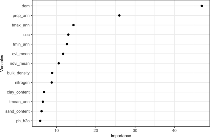
Variable importance scores (Impurity importance) from the regional Random Forest trend model
The spatial dependence structure of the residuals, obtained after fitting the regional trend model to the training data, was modeled using an exponential variogram (Fig. 7). The fitted model indicates that spatial dependence decreases with increasing distance and becomes negligible beyond approximately \(2\hspace{0.17em}km\). The short range (approximately \(2\hspace{0.17em}km\)) implies that the residual spatial autocorrelation is localized. Furthermore, the high nugget-to-sill ratio (\(96.4\mathrm{\%}\)) suggests that a substantial portion of the residual variability occurs at very short distances, potentially due to measurement noise or unresolved fine-scale spatial processes.
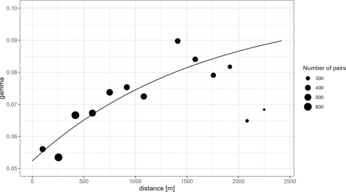
Residual variogram
Table 2 summarizes the predictive performance of the regional trend Random Forest (RF) model and the regional RFRK model, evaluated using a nested cross-validation procedure. On the regional scale, the Random Forest trend model achieved an R \({ }^{2}\) of \(0.63\) (RMSE = \(0.27\mathrm{\%}\)), while the RFRK model moderately improved performance (R \({ }^{2}=0.66\), RMSE = \(0.26\mathrm{\%}\)), indicating that the inclusion of residual spatial interpolation moderately contributes to regional predictions. Similar performance results using RFRK at the regional scale were also obtained in the study conducted by Kmoch et al. (2025).
From regional to field scale
Validation of the no-refitting RFRK strategy
To support the assumption that newly acquired field-level observations can be incorporated into the regional RFRK framework without refitting the global trend model, an experiment was conducted to evaluate the performance of different modeling strategies. The objective of this experiment was to compare how the inclusion of additional field-level observations influences the prediction accuracy under alternative modeling approaches. Specifically, three models were tested on selected fields (Fig. 8): (i) the standard regional RF trend model, (ii) the regional RF trend model augmented with new observations and refitted, and (iii) the regional RFRK model with additional observations incorporated exclusively in the geostatistical residual interpolation step, without refitting the trend model.

Residual plots for the field ID = 47. Regional RF model (left); refited regional RF model + samples (middle); RFRK model + samples without refiting (right)
The analysis considered both the distribution of residuals and the RMSE. As shown in Fig. 8, the regional trend model tends to significantly overestimate SOC values, as indicated by large negative residuals and relatively high RMSE (\(0.30\mathrm{\%}\) SOC). Incorporating additional observations and refitting the RF trend model improves prediction accuracy, reducing the RMSE to \(0.18\mathrm{\%}\) SOC. However, closer inspection of the spatial distribution of residuals reveals that this improvement is largely localized around the newly added observations. In contrast, the RFRK model with additional samples—without refitting either the trend model or the variogram—achieves both a substantial reduction in residual magnitudes (RMSE = \(0.19\mathrm{\%}\) SOC) and a more balanced spatial distribution of residuals across the field. The positive and negative residuals are more evenly distributed. This shows that when the number of additional field-level samples is small relative to the size of the training dataset used to construct the regional RFRK model—as is typically the case—the omission of a refitting step does not substantially affect the global trend representation, thus supporting the validity of the proposed approach.
Effects of targeted sampling
Sample selection within a field can be conducted randomly or according to predefined rules designed to capture spatial variability. Because random sampling does not rely on prior information about spatial patterns, it may result in favorable or unfavorable sampling configurations. For this reason, an important objective of this study was to evaluate how severe prediction errors can become under unfavorable sampling configurations and how much improvement can be achieved using the proposed targeted sampling strategy.
Figure 9 illustrates how RMSE (red) and SSIM (blue) evolve as additional local samples are incorporated into the pure regional model for representative fields (IDs 47, 120, 49, and 57). The samples were selected using the proposed sampling strategy. The primary purpose of these plots is to identify the optimal number of samples required for the regional model to approach the performance of the best-case scenario, in which all available observations are included. This was assessed by visual inspection of the curves for each field, focusing on the point at which the RMSE and SSIM values begin to stabilize.

Changes in RMSE and SSIM values based on different samples added to the pure-regional model for Fields ID = 47, 120, 49, and 57
The optimal number of field-level samples appears to be highly case-specific. In most fields, the prediction accuracy stabilized after the inclusion of several observations, as indicated by the flattening of the RMSE and SSIM curves. Only a small number of fields exhibited a monotonic improvement, where accuracy continued to increase with additional samples. The proposed number of samples ranged from \(2\) to \(13\), with an average of approximately four samples per field (see Table 3). Consequently, for the subsequent analyzes presented in this study, a subset of four samples was adopted as a representative configuration for the targeted sampling.
Importantly, no systematic relationship was observed between the field area and the optimal number of samples, suggesting that field size alone is not a reliable indicator to determine sampling density. Instead, the effectiveness of additional samples appears to depend largely on the spatial configuration of observations within the field, as clustered and uniformly distributed sampling patterns capture within-field variability with different efficiency.
Table 3 summarizes the field-level characteristics together with the corresponding RMSE and MDC values obtained for four prediction scenarios: the pure regional model, the best-possible scenario, the proposed four-sample scenario and the worst-performing four-sample scenario. The table is ordered according to the RMSE of the best-possible scenario, from lowest to highest, facilitating comparison of prediction performance across fields with increasing prediction difficulty. Mean values are reported in the final row of the table to provide a summary across all fields.
Figure 10 compares the RMSE values across fields, sorted by the best-possible scenario. The results highlight substantial variability in prediction accuracy among fields and demonstrate that the proposed four-sample strategy closely approaches the best-possible performance in many cases, while clearly outperforming the pure regional model. In particular, the pure regional model exhibits pronounced error peaks in several fields, indicating the importance of incorporating field-level observations. Several exceptions are also evident, such as Fields 83 and 132, where the best-possible scenario does not yield the lowest RMSE, suggesting potential inconsistencies related to sampling configuration or local variability.

Comparison of RMSE values across fields, sorted by the best-possible scenario. Each field is labeled with its ID and number of samples and sampling layout in parentheses. Colors indicate prediction scenarios: red—regional model without field observations; green—proposed four-sample strategy; black—best-possible scenario using all available observations
The results show that when the pure regional model is applied directly at the field scale, without incorporating field-specific observations, the predictive accuracy remains limited, with an average RMSE of \(0.24\mathrm{\%}\) between fields. This limitation becomes particularly evident in several fields where pronounced RMSE peaks are observed, notably for fields with IDs 142, 60, 124 and 137 (see Fig. 10). In these cases, the proposed four-sample scenario leads to a substantial reduction in RMSE, producing prediction accuracies that are very close to those obtained in the best-possible scenario where all observations are included. This behavior is consistent with the characteristics of the fitted residual variogram, which exhibits a short spatial range of approximately \(2\hspace{0.25em}\mathrm{k}\mathrm{m}\) and a high nugget-to-sill ratio (\(96.4\)%), indicating that most residual variability occurs at very short distances. These results indicate that the regional model alone provides a reasonable baseline prediction accuracy at the field scale, but it is unable to capture fine-scale spatial variability within fields without additional local observations.
The mean values reported in Table 3 clearly illustrate the substantial improvements when field-level observations are incorporated into the regional model. The best-case scenario, where all observations are included, achieves the lowest mean RMSE (\(0.17\)% SOC), while the proposed four-sample strategy produces a very similar result (\(0.18\)% SOC). These results indicate that the targeted sampling approach captures most of the predictive benefit of the full-observation scenario while using only a small subset of samples. The prediction accuracy achieved is comparable to values reported in previous field-scale SOC mapping studies. For example, Žı́žala et al. (2024) evaluated several covariate-based sampling strategies for Random Forest models and reported RMSE values that typically range between \(0.15\) and \(0.25\) SOC units, depending on the sampling design and sample size.
In contrast, the worst four-sample scenario results in a markedly higher mean RMSE (\(0.28\)), even exceeding the error of the pure regional model. Such behavior may arise when limited sample subsets contain high-leverage observations that are not representative of the broader within-field variability, even when they are spatially well distributed across the field. In these cases, local kriging predictions may become dominated by such observations, leading to biased SOC estimates that do not accurately represent the overall spatial pattern across the field. These results highlight the potential loss of predictive accuracy caused by poorly selected sampling locations, demonstrating that an uninformed sampling design can degrade model performance beyond that of the regional model alone.
The proposed four-sample configuration outperforms the pure regional model in \(23\) out of \(28\) fields. In the remaining cases, the pure regional model even outperforms the best-case scenario. This can be attributed to unfavorable initial sampling configurations, such as transect-based layouts and clustered random sampling, which are characteristic of these fields. Since the experiment was designed to select four samples only from the available observations, the proposed methodology was constrained by the existing spatial distribution of the samples and was therefore unable to identify an optimal sampling configuration in these cases. Consequently, the effectiveness of the proposed sampling strategy in this study is limited when the initial sampling design does not adequately represent the variability within the field. In contrast, the benefit of targeted sampling becomes much more pronounced in fields with higher within-field SOC variability and a more representative sampling distribution.
Figure 11 presents prediction maps for four representative fields, where each row compares three scenarios: the best-possible scenario (all observations included), the proposed-sample scenario (samples selected using the proposed strategy), and the worst-performing scenario (the subset of samples producing the highest prediction error). The corresponding RMSE and SSIM values are also reported for each field. In addition to numerical accuracy metrics, the figure illustrates how different sampling scenarios influence spatial prediction patterns across fields, highlighting variations in map structure and local spatial features that may arise under alternative sampling designs.

Sampling scenarios for fields ID = 47, 120, 49, and 57. For each field, three raster prediction maps are shown from left to right: (1) best-possible scenario—all samples from the field added to the pure-regional model; (2) proposed-sampling scenario—four samples selected based on the Productivity Index and standard prediction error from the regional trend model; and (3) worst-performing scenario—four samples (among all combinations of four samples) that yield the highest RMSE
Across the four representative fields, the best-possible and proposed four-sample scenarios generally produced similar spatial patterns and prediction accuracy, while the worst-performing scenarios often resulted in strong over- or underestimation. The results also show that SSIM primarily reflects similarity in spatial structure rather than absolute prediction levels. Consequently, scenarios with visually different SOC magnitudes can still achieve similar SSIM values if the spatial pattern is preserved. In addition, figure also demonstrates that the worst-performing sampling configuration is not necessarily clustered within a single part or along one side of the field. In some cases, the subset that produces the highest prediction error remains relatively well distributed across the entire field.
In summary, the results obtained highlight an important distinction between model calibration sampling and model update sampling. Although studies such as Žı́žala et al. (2024) primarily focus on sampling strategies to calibrate field-scale models from scratch, our results demonstrate that, when a reliable regional model is already available, a small number of strategically selected local observations can effectively reduce the risk of misleading sampling configurations while maintaining accuracy very close to the best-case scenario in which all field-level observations are incorporated.
Implications for SOC monitoring and MRV systems
A central challenge in SOC crediting is that the expected annual gain in SOC is often small relative to the spatial and temporal variability of the soil itself. As a result, the practical value of any monitoring, reporting, and verification (MRV) system depends not only on analytical accuracy but also on whether the monitoring design can detect changes that are sufficiently small, sufficiently fast, and with sufficiently high confidence to support carbon credit issuance. The literature consistently shows that conventional repeated soil sampling can detect changes in SOC, but its performance is strongly constrained by the heterogeneity of the field, the sampling depth, the uncertainty of the bulk density, and the time interval between measurements. Smith (2004), using a model-based analysis of SOC dynamics, showed that even under relatively favorable conditions a detectable change may require several years: in experiments with \(20\)–\(25\)% increases in C inputs, SOC change could be detected after approximately \(6\)–\(10\) years only if the monitoring system was capable of detecting a \(3\)% change in background SOC, whereas no detection was expected when the monitoring system could resolve only a \(15\)% change. Similarly, Schrumpf et al. (2011) reported that with \(100\) sampling points, the minimum detectable differences in the upper \(10\hspace{0.25em}\mathrm{c}\mathrm{m}\) were approximately \(105\pm 28\hspace{0.25em}\mathrm{g}\hspace{0.25em}\mathrm{C}\hspace{0.25em}{\mathrm{m}}^{-2}\) in cropland, \(206\pm 64\hspace{0.25em}\mathrm{g}\hspace{0.25em}\mathrm{C}\hspace{0.25em}{\mathrm{m}}^{-2}\) in grassland and \(246\pm 64\hspace{0.25em}\mathrm{g}\hspace{0.25em}\mathrm{C}\hspace{0.25em}{\mathrm{m}}^{-2}\) in forest soils, concluding that detectable change in SOC commonly requires \(2\)–\(15\) years even in stone-poor soils.
Evidence from monitoring networks further confirms that detectability is primarily a sampling-design problem. Gubler et al. (2019), analyzing \(25\) years of repeated observations in Swiss croplands, estimated a minimum detectable change (MDC) of \(0.35\)% year \({ }^{-1}\) in relative terms, highlighting that more frequent resampling, better characterization of bulk density variability, and the use of equivalent soil mass approaches can improve statistical power and reduce the minimum detectable change, while sparse repeated sampling offers limited ability to detect long-term SOC trends. At the farm scale, Deluz et al. (2020) showed that improved composite sampling can substantially reduce MDC: for an X-shaped sampling trajectory with \(20\) subsamples, the average MDC was \(0.10\)% SOC, corresponding to about \(2.7\hspace{0.25em}\mathrm{t}\hspace{0.25em}\mathrm{C}\hspace{0.25em}{\mathrm{ha}}^{-1}\) in the layer \(0\) – \(20\hspace{0.25em}\mathrm{c}\mathrm{m}\), although the field-specific range remained substantial (\(0.07\) – \(0.15\) % SOC). They further concluded that a \(20\)-aliquot composite represented a practical compromise between the monitoring effort and the sensitivity.
In this context, the results of our study provide an important complementary perspective. The values reported in Table 3 indicate that the proposed four-sample strategy achieves MDC levels (\(\approx 0.50\mathrm{\%}\) SOC) very close to those obtained in the full-observation scenario (\(\approx 0.47\mathrm{\%}\) SOC), while substantially improving over unfavorable sampling configurations (\(\approx 0.78\mathrm{\%}\) SOC). Although previous studies primarily aimed to reduce MDC by increasing sampling density or using composite sampling designs, our results demonstrate that the number of samples can be substantially reduced through optimized spatial placement while maintaining comparable model sensitivity and significantly improving performance relative to unfavorable sampling configurations. Furthermore, the obtained MDC values remain relatively high compared to the magnitude of typical annual SOC changes, indicating that the reliable detection of short-term SOC changes at the field scale remains a challenge. Nevertheless, the results still provide valuable insight into the relative sensitivity of different sampling strategies and suggest that the proposed framework is more suitable to identify medium- to long-term SOC trends than year-to-year changes, which is consistent with previous findings (Schrumpf et al., 2011; Smith, 2004). Although fundamental limitations in detectability remain, the proposed approach still represents a practical pathway toward more efficient and scalable MRV systems, particularly in smallholder-dominated agricultural systems where dense sampling is not feasible.
Limitations and future perspectives
Although the proposed framework demonstrated promising results to improve field-scale SOC prediction, several aspects should be considered when interpreting the findings and assessing their broader applicability. The spatial distribution of SOC observations across Vojvodina remains relatively sparse and uneven, which may limit the ability of the regional model to fully capture spatial variability in SOC. In addition, the environmental covariates used to construct the regional model originated from multiple data sources with different native spatial resolutions and were therefore resampled to a common resolution of \(30\hspace{0.25em}\mathrm{m}\). Although suitable for regional modeling, this resolution may still be insufficient for representing fine-scale variability at the field scale.
Another important consideration relates to the spatial configuration of field observations. Sampling layouts varied substantially between fields, ranging from relatively uniform spatial coverage to clustered or transect-based arrangements. Although such variability is useful for assessing the effects of realistic sampling scenarios, in this study it constrained the ability of the methodology to identify fully representative sampling scenarios, particularly when observations covered only a limited portion of the field.
It should be noted that the MDC values obtained were calculated solely from spatial prediction errors, while the uncertainties associated with the SOC measurements themselves were assumed to be negligible. Consequently, the reported MDC values should be interpreted primarily as indicators of the relative sensitivity of different sampling strategies rather than as absolute detection thresholds.
Future research should therefore focus on evaluating the framework using denser and more systematically distributed observations, as well as higher-resolution environmental covariates better suited for field-scale applications. Additional research is also needed to assess the applicability of the proposed approach within operational SOC monitoring and carbon farming MRV frameworks.
Conclusion
This study demonstrates that regional SOC prediction models can be effectively enhanced on a field scale through the integration of a small number of strategically selected local observations. Although incorporating all field-level measurements provides the highest prediction accuracy, our results show that carefully selected subsets of observations can achieve very similar performance with substantially fewer samples.
The proposed productivity-based targeted sampling strategy significantly improves field-level predictions compared to the pure regional model. On average, the prediction error was reduced from a RMSE of \(0.24\mathrm{\%}\) SOC for the regional model to \(0.18\mathrm{\%}\) SOC using only four strategically selected samples, approaching the precision of the full-observation scenario (RMSE = \(0.17\mathrm{\%}\) SOC). These improvements are particularly evident in fields with representative initial sampling configurations and higher within-field SOC variability, where regional models alone cannot fully capture fine-scale spatial heterogeneity.
The results highlight the value of integrating regional prediction models with targeted sampling strategies, as even a spatially representative random sampling arrangement can still lead to misleading SOC assessments across the field. Indicators derived from multi-year NDVI time series provide spatially meaningful information on persistent productivity patterns, enabling the identification of informative sampling locations within agricultural fields. In general, the proposed framework can substantially improve field-scale SOC estimates while minimizing sampling effort and reducing the risk of unfavorable sampling configurations. This approach offers a practical and scalable solution for carbon farming and soil carbon monitoring systems, where reliable SOC estimates must be achieved under operational constraints on sampling intensity.
Data availability
The complete dataset and source code are publicly available at the link: https://github.com/pejovic/Data-driven-targeted-sampling-paper and https://doi.org/10.5281/zenodo.19511914
References
Amelung, W., Bossio, D., de Vries, W., Kögel-Knabner, I., Lehmann, J., Amundson, R., Bol, R., Collins, C., Lal, R., Leifeld, J., Minasny, B., Pan, G., Paustian, K., Rumpel, C., Sanderman, J., van Groenigen, J. W., Mooney, S., van Wesemael, B., Wander, M., & Chabbi, A. (2020). Towards a global-scale soil climate mitigation strategy. Nature Communications, 11(1), Article 5427. https://doi.org/10.1038/s41467-020-18887-7
Batjes, N. H. (2019). Technologically achievable soil organic carbon sequestration in world croplands and grasslands. Land Degradation & Development, 30, 25–32. https://doi.org/10.1002/ldr.3209
Batjes, N. H., Ceschia, E., Heuvelink, G. B. M., Demenois, J., Maire, G., Cardinael, R., Arias-Navarro, C., & van Egmond, F. (2024). Towards a modular, multi-ecosystem monitoring, reporting and verification (MRV) framework for soil organic carbon stock change assessment. Carbon Management, 15(1), Article 2410812. https://doi.org/10.1080/17583004.2024.2410812
Breiman, L. (2001). Random forests. Machine Learning, 45(1), 5–32. https://doi.org/10.1023/A:1010933404324
Brus, D. J. (2019). Sampling for digital soil mapping: A tutorial supported by r scripts. Geoderma, 338, 464–480. https://doi.org/10.1016/j.geoderma.2018.07.036
Chambers, A., Lal, R., & Paustian, K. (2016). Soil carbon sequestration potential of US croplands and grasslands: Implementing the 4 per thousand initiative. Journal of Soil and Water Conservation, 71(3), 68A-74A. https://doi.org/10.2489/jswc.71.3.68A
Deluz, C., Nussbaum, M., Sauzet, O., Gondret, K., & Boivin, P. (2020). Evaluation of the potential for soil organic carbon content monitoring with farmers. Frontiers in Environmental Science. https://doi.org/10.3389/fenvs.2020.00113
Deng, Y., Zhang, X., Yang, Y., Cao, J., Yin, L., & Zhang, B. (2025). Enhancing soil organic carbon prediction in coastal farmlands using multi-source remote sensing data and machine learning. Smart Agricultural Technology, 11, Article 101059. https://doi.org/10.1016/j.atech.2025.101059
Dhawale, N. M., Adamchuk, V. I., Prasher, S. O., & Viscarra Rossel, R. A. (2021). Evaluating the precision and accuracy of proximal soil vis–NIR sensors for estimating soil organic matter and texture. Soil Systems, 5(3), Article 48. https://doi.org/10.3390/soilsystems5030048
Dhawale, N. M., Adamchuk, V. I., Prasher, S. O., Dutilleul, P. R. L., & Ferguson, R. B. (2014). Spatially constrained geospatial data clustering for multilayer sensor-based measurements. International Archives of the Photogrammetry, Remote Sensing and Spatial Information Sciences, XL–2, 187–190. https://doi.org/10.5194/isprsarchives-XL-2-187-2014
Djurović, P. (2022). Geomorphological characteristics of Serbia. In E. Manić, V. Nikitović, & P. Djurović (Eds.), The geography of Serbia: Nature, people, economy (pp. 85–98). Springer International Publishing. https://doi.org/10.1007/978-3-030-74701-5_7
Drusch, M., Del Bello, U., Carlier, S., Colin, O., Fernández, V., Gascon, F., Hoersch, B., Isola, C., Laberinti, P., Martimort, P., Meygret, A., Spoto, F., Sy, O., Marchese, F., & Bargellini, P. (2012). Sentinel-2: ESA’s optical high-resolution mission for GMES operational services. Remote Sensing of Environment, 120, 25–36. https://doi.org/10.1016/j.rse.2011.11.026
Etezadi, H., Bouroubi, Y., Adamchuk, V., Leduc, M., Gasser, M.-O., & Saifuzzaman, M. (2026). A multi-scale framework for predicting continuous soil properties using ranked sentinel-2 images and zone-level soil data: From a farm case study to a regional application. Smart Agricultural Technology, 14, Article 102035. https://doi.org/10.1016/j.atech.2026.102035
Falk, M. G., Denham, R. J., & Mengersen, K. L. (2011). Spatially stratified sampling using auxiliary information for geostatistical mapping. Environmental and Ecological Statistics, 18(1), 93–108. https://doi.org/10.1007/s10651-009-0122-3
Gubler, A., Wächter, D., Schwab, P., Müller, M., & Keller, A. (2019). Twenty-five years of observations of soil organic carbon in Swiss croplands showing stability overall but with some divergent trends. Environmental Monitoring and Assessment, 191(5), 277. https://doi.org/10.1007/s10661-019-7435-y
Hengl, T., Heuvelink, G. B. M., & Rossiter, D. G. (2007). About regression-kriging: From equations to case studies. Computers & Geosciences, 33(10), 1301–1315. https://doi.org/10.1016/j.cageo.2007.05.001
Hengl, T., Heuvelink, G. B. M., & Stein, A. (2004). A generic framework for spatial prediction of soil variables based on regression-kriging. Geoderma, 120(1), 75–93. https://doi.org/10.1016/j.geoderma.2003.08.018
Hengl, T., Nussbaum, M., Wright, M. N., Heuvelink, G. B. M., Gräler, B., & Svoray, T. (2018). Random forest as a generic framework for predictive modeling of spatial and spatio-temporal variables. PeerJ, 6, Article e5518. https://doi.org/10.7717/peerj.5518
Ho, V. H., Morita, H., Bachofer, F., & Ho, T. H. (2024). Random forest regression kriging modeling for soil organic carbon density estimation using multi-source environmental data in central Vietnamese forests. Modeling Earth Systems and Environment, 10(6), 7137–7158. https://doi.org/10.1007/s40808-024-02158-1
Jangir, A., Nogiya, M., Yadav, B., Malav, L. C., Moharana, P. C., Meena, R. L., Sharma, R. P., Tiwari, G., Dash, B., Naitam, R., Vasu, D., Mina, B. L., & Patil, N. G. (2026). Regional-scale predictive mapping of soil organic carbon in south Gujarat, India using machine learning algorithms. Environmental Monitoring and Assessment, 198(4), 325. https://doi.org/10.1007/s10661-026-15158-8
Kaya, F., Keshavarzi, A., Francaviglia, R., Kaplan, G., Başayiğit, L., & Dedeoğlu, M. (2022). Assessing machine learning-based prediction under different agricultural practices for digital mapping of soil organic carbon and available phosphorus. Agriculture, 12(7), Article 1062. https://doi.org/10.3390/agriculture12071062
Khaledian, Y., & Miller, B. A. (2020). Selecting appropriate machine learning methods for digital soil mapping. Applied Mathematical Modelling, 81, 401–418. https://doi.org/10.1016/j.apm.2019.12.016
Kmoch, A., Harrison, C. T., Choi, J., & Uuemaa, E. (2025). Spatial autocorrelation in machine learning for modelling soil organic carbon. Ecological Informatics, 86, Article 103057. https://doi.org/10.1016/j.ecoinf.2025.103057
Krstajic, D., Buturovic, L. J., Leahy, D. E., & Thomas, S. (2014). Cross-validation pitfalls when selecting and assessing regression and classification models. Journal of Cheminformatics, 6, Article 10. https://doi.org/10.1186/1758-2946-6-10
Kumar, N., Velmurugan, A., Hamm, N. A. S., & Dadhwal, V. K. (2018). Geospatial mapping of soil organic carbon using regression kriging and remote sensing. Journal of the Indian Society of Remote Sensing, 46(5), 705–716. https://doi.org/10.1007/s12524-017-0738-y
Lal, R. (2004). Soil carbon sequestration impacts on global climate change and food security. Science, 304, 1623–1627. https://doi.org/10.1126/science.1097396
Lamichhane, S., Kumar, L., & Wilson, B. (2019). Digital soil mapping algorithms and covariates for soil organic carbon mapping and their implications: A review. Geoderma, 352, 395–413. https://doi.org/10.1016/j.geoderma.2019.05.031
Li, X., Shen, T., Garcia, C. L., et al. (2025). A 30-meter resolution global land productivity dynamics dataset from 2013 to 2022. Scientific Data, 12, Article 555. https://doi.org/10.1038/s41597-025-04883-3
Ma, T., Brus, D. J., Zhu, A.-X., Zhang, L., & Scholten, T. (2020). Comparison of conditioned latin hypercube and feature space coverage sampling for predicting soil classes using simulation from soil maps. Geoderma, 370, Article 114366. https://doi.org/10.1016/j.geoderma.2020.114366
Mair, M. M., Kattwinkel, M., Jakoby, O., & Hartig, F. (2020). The minimum detectable difference (MDD) concept for establishing trust in nonsignificant results: A critical review. Environmental Toxicology and Chemistry, 39, 2109–2123. https://doi.org/10.1002/etc.4847
Minasny, B., Malone, B. P., McBratney, A. B., Angers, D. A., Arrouays, D., Chambers, A., Chaplot, V., Chen, Z.-S., Cheng, K., Das, B. S., Field, D. J., Gimona, A., Hedley, C. B., Hong, S. Y., Mandal, B., Marchant, B. P., Martin, M., McConkey, B. G., Mulder, V. L., … Winowiecki, L. (2017). Soil carbon 4 per mille. Geoderma, 292, 59–86. https://doi.org/10.1016/j.geoderma.2017.01.002
Minasny, B., & McBratney, A. B. (2006). A conditioned latin hypercube method for sampling in the presence of ancillary information. Computers & Geosciences, 32(9), 1378–1388. https://doi.org/10.1016/j.cageo.2005.12.009
Parvizi, Y., & Fatehi, S. (2025). Geospatial digital mapping of soil organic carbon using machine learning and geostatistical methods in different land uses. Scientific Reports, 15(1), Article 4449. https://doi.org/10.1038/s41598-025-88062-9
Paul, C., Bartkowski, B., Dönmez, C., Don, A., Mayer, S., Steffens, M., Weigl, S., Wiesmeier, M., Wolf, A., & Helming, K. (2023). Carbon farming: Are soil carbon certificates a suitable tool for climate change mitigation? Journal of Environmental Management, 330, Article 117142. https://doi.org/10.1016/j.jenvman.2022.117142
Paustian, K., Collier, S., Baldock, J., Burgess, R., Creque, J., DeLonge, M., Dungait, J., Ellert, B., Frank, S., Goddard, T., Govaerts, B., Grundy, M., Henning, M., Izaurralde, R. C., Madaras, M., McConkey, B., Porzig, E., Rice, C., Searle, R., … Jahn, M. (2019). Quantifying carbon for agricultural soil management: From the current status toward a global soil information system. Carbon Management, 10(6), 567–587. https://doi.org/10.1080/17583004.2019.1633231
Pejović, M., Nikolić, M., Heuvelink, G. B. M., Hengl, T., Kilibarda, M., & Bajat, B. (2018). Sparse regression interaction models for spatial prediction of soil properties in 3D. Computers & Geosciences, 118, 1–13. https://doi.org/10.1016/j.cageo.2018.05.008
Petropoulos, T., Benos, L., Busato, P., Kyriakarakos, G., Kateris, D., Aidonis, D., & Bochtis, D. (2025). Soil organic carbon assessment for carbon farming: A review. Agriculture. https://doi.org/10.3390/agriculture15050567
Pouladi, N., Gholizadeh, A., Khosravi, V., & Borůvka, L. (2023). Digital mapping of soil organic carbon using remote sensing data: A systematic review. CATENA, 232, Article 107409. https://doi.org/10.1016/j.catena.2023.107409
Sachin, M. L., Yogananda, S. B., Pruthviraj, Pravalika, K. M., & Roopa, M. N. (2026). Advances in soil carbon monitoring and management: Tools and strategies for climate-smart and sustainable agriculture. Environmental Monitoring and Assessment, 198(3), 283. https://doi.org/10.1007/s10661-026-15106-6
Saurette, D. D., Heck, R. J., Gillespie, A. W., Berg, A. A., & Biswas, A. (2024). Sample size optimization for digital soil mapping: An empirical example. Land, 13(3), Article 365. https://doi.org/10.3390/land13030365
Schillaci, C., Yunta, F., Scarpa, S., Wojda, P., Vieira, D., Panagos, P., & Jones, A. (2026). Enhancing the SDG 15.3.1 land-cover transition matrix using multidecadal vegetation indicators. Journal of Land Use Science, 21(1), 163–183. https://doi.org/10.1080/1747423X.2026.2638216
Schmidt, K., Behrens, T., Daumann, J., Ramirez-Lopez, L., Werban, U., Dietrich, P., & Scholten, T. (2014). A comparison of calibration sampling schemes at the field scale. Geoderma, 232–234, 243–256. https://doi.org/10.1016/j.geoderma.2014.05.013
Schmidt, M. W. I., Torn, M. S., Abiven, S., Dittmar, T., Guggenberger, G., Janssens, I. A., Kleber, M., Kögel-Knabner, I., Lehmann, J., Manning, D. A. C., Nannipieri, P., Rasse, D. P., Weiner, S., & Trumbore, S. E. (2011). Persistence of soil organic matter as an ecosystem property. Nature, 478(7367), 49–56. https://doi.org/10.1038/nature10386
Schrumpf, M., Schulze, E. D., Kaiser, K., & Schumacher, J. (2011). How accurately can soil organic carbon stocks and stock changes be quantified by soil inventories? Biogeosciences, 8(5), 1193–1212. https://doi.org/10.5194/bg-8-1193-2011
Sekulić, A., Kilibarda, M., Heuvelink, G. B. M., Nikolić, M., & Bajat, B. (2020a). Random forest spatial interpolation. Remote Sensing, 12(10), Article 1687. https://doi.org/10.3390/rs12101687
Sekulić, A., Kilibarda, M., Protić, D., & Bajat, B. (2020b). MeteoSerbia1km: The first daily gridded meteorological dataset at a 1-km spatial resolution across serbia for the 2000–2019 period (Version 1.0.0) [Dataset]. Zenodo. https://doi.org/10.5281/zenodo.4058167
Sekulić, P., Ninkov, J., Hristov, N., Vasin, J., Šeremešić, S., & Zeremski-Škorić, T. (2010). Organic matter content in vojvodina soils and the possibility of using harvest residues as renewable source of energy. (in Serbian), Ratarstvo i Povrtarstvo/Field and Vegetable Crops Research, 47, 591–598. from: https://scindeks-clanci.ceon.rs/data/pdf/1821-3944/2010/1821-39441002591S.pdf
Shamrikova, E. V., Kondratenok, B. M., Tumanova, E. A., Vanchikova, E. V., Lapteva, E. M., Zonova, T. V., Lu-Lyan-Min, E. I., Davydova, A. P., Libohova, Z., & Suvannang, N. (2022). Transferability between soil organic matter measurement methods for database harmonization. Geoderma, 412, Article 115547. https://doi.org/10.1016/j.geoderma.2021.115547
Simbahan, G. C., & Dobermann, A. (2006). Sampling optimization based on secondary information and its utilization in soil carbon mapping. Geoderma, 133(3), 345–362. https://doi.org/10.1016/j.geoderma.2005.07.020
Smith, P. (2004). How long before a change in soil organic carbon can be detected? Global Change Biology, 10(11), 1878–1883. https://doi.org/10.1111/j.1365-2486.2004.00854.x
Talebi, H., Peeters, L. J. M., Otto, A., & Tolosana-Delgado, R. (2022). A truly spatial random forests algorithm for geoscience data analysis and modelling. Mathematical Geosciences, 54(1), 1–22. https://doi.org/10.1007/s11004-021-09946-w
Van Hoof, S. (2023). Climate change mitigation in agriculture: Barriers to the adoption of carbon farming policies in the EU. Sustainability. https://doi.org/10.3390/su151310452
Vasin, J., Ninkov, J., Zeremski, T., Milić, S., Jakšić, S., & Živanov, M. (2021). Soils of vojvodina – quality and organic matter. (in Serbian) Racionalno Korišćenje Zemljišta i Voda u Srbiji, 133–138. https://hdl.handle.net/21.15107/rcub_dais_13182
Wadoux, A. M. J. C., Dobarco, M. R., Malone, B., Minasny, B., McBratney, A. B., & Searle, R. (2023). Baseline high-resolution maps of organic carbon content in Australian soils. Scientific Data. https://doi.org/10.1038/s41597-023-02056-8
Wadoux, A.M.J.-C., Brus, D. J., & Heuvelink, G. B. M. (2019). Sampling design optimization for soil mapping with random forest. Geoderma, 355, Article 113913. https://doi.org/10.1016/j.geoderma.2019.113913
Wadoux, A.M.J.-C., Minasny, B., & McBratney, A. B. (2020). Machine learning for digital soil mapping: Applications, challenges and suggested solutions. Earth-Science Reviews, 210, Article 103359. https://doi.org/10.1016/j.earscirev.2020.103359
Wang, S., Guan, K., Zhang, C., Lee, D., Margenot, A. J., Ge, Y., Peng, J., Zhou, W., Zhou, Q., & Huang, Y. (2022). Using soil library hyperspectral reflectance and machine learning to predict soil organic carbon: Assessing potential of airborne and spaceborne optical soil sensing. Remote Sensing of Environment, 271, Article 112914. https://doi.org/10.1016/j.rse.2022.112914
Wang, Z., Bovik, A. C., Sheikh, H. R., & Simoncelli, E. P. (2004). Image quality assessment: From error visibility to structural similarity. IEEE Transactions on Image Processing, 13(4), 600–612. https://doi.org/10.1109/TIP.2003.819861
Webster, R., & Oliver, M. A. (2007). Geostatistics for environmental scientists. John Wiley & Sons. https://doi.org/10.1002/9780470517277
Witjes, M., Parente, L., Križan, J., Hengl, T., Antonić, L., & Wang, J. (2023). Ecodatacube.eu: Analysis-ready open environmental data cube for europe. PeerJ, 11, e15478. https://doi.org/10.7717/peerj.15478
Worsham, L., Markewitz, D., Nibbelink, N. P., & West, L. T. (2012). A comparison of three field sampling methods to estimate soil carbon content. Forensic Science, 58(5), 513–522. https://doi.org/10.5849/forsci.11-084
Žı́žala, D., Princ, T., Skála, J., Juřicová, A., Lukas, V., Bohovic, R., Zádorová, T., & Minařı́k, R. (2024). Soil sampling design matters: Enhancing the efficiency of digital soil mapping at the field scale. Geoderma Regional, 39, e00874. https://doi.org/10.1016/j.geodrs.2024.e00874
Acknowledgements
This study was supported by the Ministry of Education, Science and Technological Development of the Republic of Serbia under research project No. 200092, and by the Open Geospatial Carbon Registry (OGCR) project funded by the European Union; Horizon Europe programme under Grant Agreement No. 101218854.
Author information
Authors and Affiliations
Contributions
All authors contributed to the study design and methodology. Conceptualization: MP, MK, DP, BB; Methodology: MP, MK, DP; Data preparation, Formal analysis, and Software: MP; Writing – original draft preparation: MP; Writing – review and editing: MK, DP, BB; Verification: MK, DP, BB. All authors read and approved the final manuscript.
Corresponding author
Ethics declarations
Ethics approval
All authors have read, understood, and adhered as applicable to the statement on “Ethical responsibilities of Authors” as found in the Instructions for Authors.
Competing interests
The authors declare no competing interests.
Additional information
Publisher's Note
Springer Nature remains neutral with regard to jurisdictional claims in published maps and institutional affiliations.
Rights and permissions
Open Access This article is licensed under a Creative Commons Attribution-NonCommercial-NoDerivatives 4.0 International License, which permits any non-commercial use, sharing, distribution and reproduction in any medium or format, as long as you give appropriate credit to the original author(s) and the source, provide a link to the Creative Commons licence, and indicate if you modified the licensed material. You do not have permission under this licence to share adapted material derived from this article or parts of it. The images or other third party material in this article are included in the article's Creative Commons licence, unless indicated otherwise in a credit line to the material. If material is not included in the article's Creative Commons licence and your intended use is not permitted by statutory regulation or exceeds the permitted use, you will need to obtain permission directly from the copyright holder. To view a copy of this licence, visit http://creativecommons.org/licenses/by-nc-nd/4.0/.
About this article
Cite this article
Pejović, M., Kilibarda, M., Protić, D. et al. Productivity-based sampling for field-scale soil organic carbon mapping: from regional models to carbon farming needs. Environ Monit Assess 198, 955 (2026). https://doi.org/10.1007/s10661-026-15793-1
Received:
Accepted:
Published:
Version of record:
DOI: https://doi.org/10.1007/s10661-026-15793-1