Data cleaning is a step in machine learning (ML) which involves identifying and removing any missing, duplicate or irrelevant data.
- Raw data (log file, transactions, audio /video recordings, etc) is often noisy, incomplete and inconsistent which can negatively impact the accuracy of model.
- The goal of data cleaning is to ensure that the data is accurate, consistent and free of errors.
- Clean datasets also important in EDA (Exploratory Data Analysis) which enhances the interpretability of data so that the right actions can be taken based on insights.
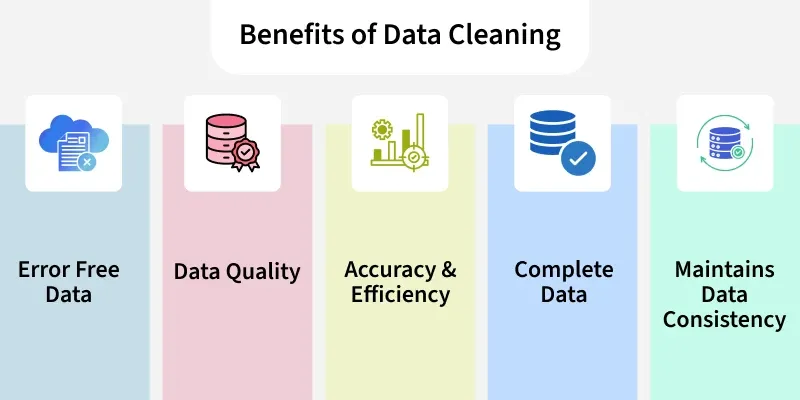 Benefits of Data Cleaning
The process begins by identifying issues like missing values, duplicates and outliers. Performing data cleaning involves a systematic process to identify and remove errors in a dataset. The following steps are essential to perform data cleaning:
- Remove Unwanted Observations: Eliminate duplicates, irrelevant entries or redundant data that add noise.
- Fix Structural Errors: Standardize data formats and variable types for consistency.
- Manage Outliers: Detect and handle extreme values that can skew results, either by removal or transformation.
- Handle Missing Data: Address gaps using imputation, deletion or advanced techniques to maintain accuracy and integrity.
Implementation for Data Cleaning
Let's understand each step for Database Cleaning using titanic dataset.
Step 1: Import Libraries and Load Dataset
We will import all the necessary libraries i.e pandas and numpy.
Python
import pandas as pd
import numpy as np

df = pd.read_csv('Titanic-Dataset.csv')
df.info()
df.head()
Output:
Step 2: Check for Duplicate Rows
df.duplicated(): Returns a boolean Series indicating duplicate rows.
Python
Output:
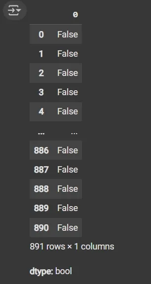 Duplicated Data
Step 3: Identify Column Data Types
- List comprehension with .dtype attribute to separate categorical and numerical columns.
- object dtype: Generally used for text or categorical data.
Python
cat_col = [col for col in df.columns if df[col].dtype == 'object']
num_col = [col for col in df.columns if df[col].dtype != 'object']

print('Categorical columns:', cat_col)
print('Numerical columns:', num_col)
Output:
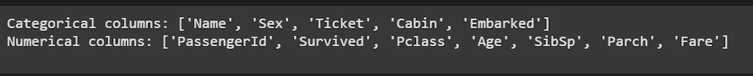 Column Data Types
Step 4: Count Unique Values in the Categorical Columns
df[numeric_columns].nunique(): Returns count of unique values per column.
Python
Output:
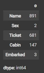 Unique Values
Step 5: Calculate Missing Values as Percentage
- df.isnull(): Detects missing values, returning boolean DataFrame.
- Sum missing across columns, normalize by total rows and multiply by 100.
Python
round((df.isnull().sum() / df.shape[0]) * 100, 2)
Output:
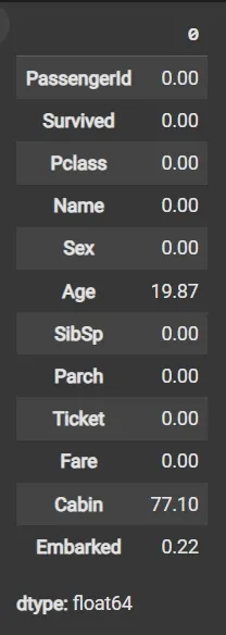 Missing Value Percentage
 Step 6: Drop Irrelevant or Data-Heavy Missing Columns
- df.drop(columns=[]): Drops specified columns from the DataFrame.
- df.dropna(subset=[]): Removes rows where specified columns have missing values.
- fillna(): Fills missing values with specified value (e.g., mean).
Python
df1 = df.drop(columns=['Name', 'Ticket', 'Cabin'])
df1.dropna(subset=['Embarked'], inplace=True)
df1['Age'].fillna(df1['Age'].mean(), inplace=True)
Step 7: Detect Outliers with Box Plot
- matplotlib.pyplot.boxplot(): Displays distribution of data, highlighting median, quartiles and outliers.
- plt.show(): Renders the plot.
Python
import matplotlib.pyplot as plt

plt.boxplot(df3['Age'], vert=False)
plt.ylabel('Variable')
plt.xlabel('Age')
plt.title('Box Plot')
plt.show()
Output:
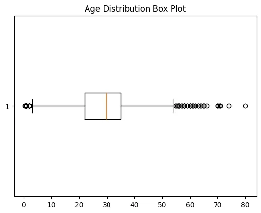 Boxplot
Step 8: Calculate Outlier Boundaries and Remove Them
- Calculate mean and standard deviation (std) using df['Age'].mean() and df['Age'].std().
- Define bounds as mean ± 2 * std for outlier detection.
- Filter DataFrame rows within bounds using Boolean indexing.
Python
mean = df1['Age'].mean()
std = df1['Age'].std()

lower_bound = mean - 2 * std
upper_bound = mean + 2 * std

df2 = df1[(df1['Age'] >= lower_bound) & (df1['Age'] <= upper_bound)]
Step 9: Impute Missing Data Again if Any
fillna() applied again on filtered data to handle any remaining missing values.
Python
df3 = df2.fillna(df2['Age'].mean())
df3.isnull().sum()
Output:
 Missing Value
Step 10: Recalculate Outlier Bounds and Remove Outliers from the Updated Data
- mean = df3['Age'].mean(): Calculates the average (mean) value of the Age column in the DataFrame df3.
- std = df3['Age'].std(): Computes the standard deviation (spread or variability) of the Age column in df3.
- lower_bound = mean - 2 * std: Defines the lower limit for acceptable Age values, set as two standard deviations below the mean.
- upper_bound = mean + 2 * std: Defines the upper limit for acceptable Age values, set as two standard deviations above the mean.
- df4 = df3[(df3['Age'] >= lower_bound) & (df3['Age'] <= upper_bound)]: Creates a new DataFrame df4 by selecting only rows where the Age value falls between the lower and upper bounds, effectively removing outlier ages outside this range.
Python
mean = df3['Age'].mean()
std = df3['Age'].std()

lower_bound = mean - 2 * std
upper_bound = mean + 2 * std

print('Lower Bound :', lower_bound)
print('Upper Bound :', upper_bound)

df4 = df3[(df3['Age'] >= lower_bound) & (df3['Age'] <= upper_bound)]
Output:
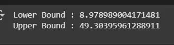 Outlier Check
Step 11: Data validation and verification
Data validation and verification involve ensuring that the data is accurate and consistent by comparing it with external sources or expert knowledge. For the machine learning prediction we separate independent and target features. Here we will consider only 'Sex' 'Age' 'SibSp', 'Parch' 'Fare' 'Embarked' only as the independent features and Survived as target variables because PassengerId will not affect the survival rate.
Python
X = df3[['Pclass','Sex','Age', 'SibSp','Parch','Fare','Embarked']]
Y = df3['Survived']
Data formatting involves converting the data into a standard format or structure that can be easily processed by the algorithms or models used for analysis. Here we will discuss commonly used data formatting techniques i.e. Scaling and Normalization.
Scaling involves transforming the values of features to a specific range. It maintains the shape of the original distribution while changing the scale. It is useful when features have different scales and certain algorithms are sensitive to the magnitude of the features. Common scaling methods include:
1. Min-Max Scaling: Min-Max scaling rescales the values to a specified range, typically between 0 and 1. It preserves the original distribution and ensures that the minimum value maps to 0 and the maximum value maps to 1.
Python
from sklearn.preprocessing import MinMaxScaler

scaler = MinMaxScaler(feature_range=(0, 1))

num_col_ = [col for col in X.columns if X[col].dtype != 'object']
x1 = X
x1[num_col_] = scaler.fit_transform(x1[num_col_])
x1.head()
Output:
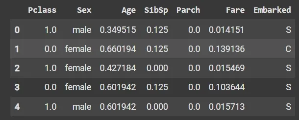 Min-Max Scaling
2. Standardization (Z-score scaling): Standardization transforms the values to have a mean of 0 and a standard deviation of 1. It centers the data around the mean and scales it based on the standard deviation. Standardization makes the data more suitable for algorithms that assume a Gaussian distribution or require features to have zero mean and unit variance.
Z = (X - μ) / σ
Where,
- X = Data
- μ = Mean value of X
- σ = Standard deviation of X
Some data cleansing tools:
- OpenRefine: A free, open-source tool for cleaning, transforming and enriching messy data with an easy-to-use interface and powerful features like clustering and faceting.
- Trifacta Wrangler: An AI-powered, user-friendly platform that helps automate data cleaning and transformation workflows for faster, more accurate preparation.
- TIBCO Clarity: A data profiling and cleansing tool that ensures high-quality, standardized and consistent datasets across diverse sources.
- Cloudingo: A cloud-based solution focused on deduplication and data cleansing, especially useful for maintaining accurate CRM data.
- IBM InfoSphere QualityStage: An enterprise-grade tool designed for large-scale, complex data quality management including profiling, matching and cleansing.
Advantages
- Improved model performance: Removal of errors, inconsistencies and irrelevant data helps the model to better learn from the data.
- Increased accuracy: Helps ensure that the data is accurate, consistent and free of errors.
- Better representation of the data: Data cleaning allows the data to be transformed into a format that better represents the underlying relationships and patterns in the data.
- Improved data quality: Improve the quality of the data, making it more reliable and accurate.
- Improved data security: Helps to identify and remove sensitive or confidential information that could compromise data security.
Disadvantages
- Time-consuming: It is very time consuming task specially for large and complex datasets.
- Error-prone: It can result in loss of important information.
- Cost and resource-intensive: It is resource-intensive process that requires significant time, effort and expertise. It can also require the use of specialized software tools.
- Overfitting: Data cleaning can contribute to overfitting by removing too much data.