NumPy Array Broadcasting with Examples
NumPy broadcasting is a powerful feature that allows you to perform arithmetic operations on arrays of different shapes and sizes. It does this by automatically replicating the smaller array along the last mismatched dimension until both arrays have the same shape.
Broadcasting is a very efficient way to perform vectorized operations, and it can be used to simplify many common numerical computing tasks. For example, you can use broadcasting to add a scalar value to all elements of an array or to multiply two arrays of different sizes element-wise.
Understanding Broadcasting in NumPy
At its core, broadcasting is NumPy’s way of making arrays with different shapes compatible with element-wise operations. Instead of manually reshaping or repeating values in arrays, NumPy automatically aligns them for you, improving both code readability and performance.
Let’s start with a basic example. Suppose we have two arrays, a and b:
import numpy as np

a = np.array([1.0, 2.0, 3.0])
b = np.array([2.0, 2.0, 2.0])
result = a * b
In this case, a and b have the same shape, so the element-wise multiplication works straightforwardly. The result is [2.0, 4.0, 6.0].
Sample:
Broadcasting a Scalar
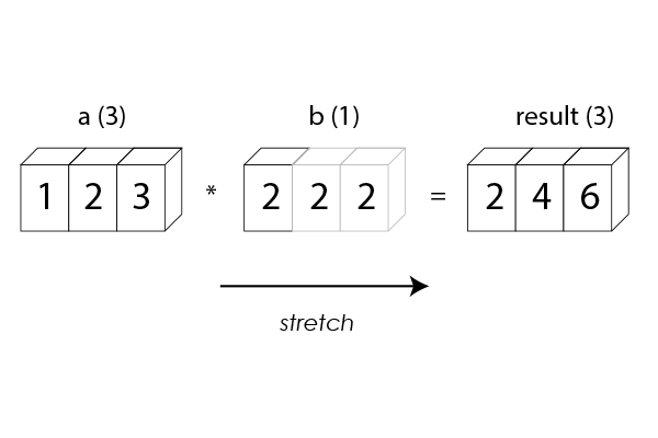
Broadcasting becomes more interesting when we introduce a scalar value. Consider this:
a = np.array([1.0, 2.0, 3.0])
b = 2.0
result = a * b
Now, b is a scalar, but NumPy automatically broadcasts it to match the shape of a. The result remains the same: [2.0, 4.0, 6.0].
The magic happens behind the scenes; NumPy efficiently operates on the scalar without creating unnecessary copies of data.
General Broadcasting Rules
To understand broadcasting fully, you need to grasp the general broadcasting rules:
NumPy compares array shapes element-wise, starting from the trailing (rightmost) dimensions.
Two dimensions are considered compatible if:
They are equal, or
One of them is 1.
If the conditions are not met, NumPy raises a ValueError, indicating incompatible shapes.
This flexibility allows NumPy to handle arrays of different shapes intelligently. Missing dimensions are assumed to have size one.
Examples of Broadcasting
Broadcasting with One-Dimensional and Two-Dimensional Arrays
a = np.array([[0.0, 0.0, 0.0],
              [10.0, 10.0, 10.0],
              [20.0, 20.0, 20.0],
              [30.0, 30.0, 30.0]])
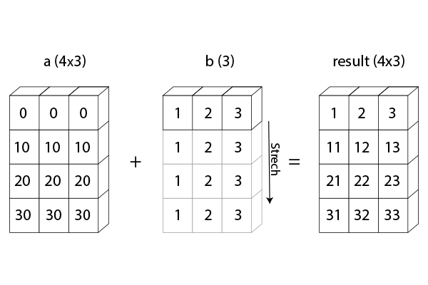
b = np.array([1.0, 2.0, 3.0])
result = a + b
In this example, b is added to each row of a, resulting in broadcasting.
Sample
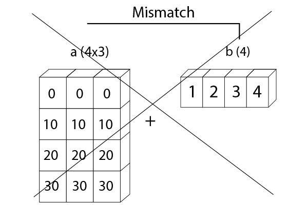
However, if we change b to have four elements:
b = np.array([1.0, 2.0, 3.0, 4.0])
result = a + b  # Raises a ValueError
The shapes are incompatible, and broadcasting fails.
Sample:
Outer Operation
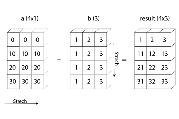
Broadcasting also simplifies outer operations. Here’s an example of outer addition between two one-dimensional arrays:
a = np.array([0.0, 10.0, 20.0, 30.0])
b = np.array([1.0, 2.0, 3.0])
result = a[:, np.newaxis] + b
The [:, np.newaxis] operation inserts a new axis into a, making it a two-dimensional array, which can then be broadcast with b.
Sample:
Conclusion
As you continue your journey with NumPy, mastering broadcasting will empower you to write more concise and readable code while optimizing computational performance. Whether you’re dealing with arrays of the same shape or combining scalars with multi-dimensional arrays, broadcasting simplifies the process, making NumPy a go-to tool for scientific computing and data manipulation tasks. With a solid understanding of broadcasting, you’re well-equipped to tackle a wide range of numerical problems and unlock the full potential of NumPy in your Python projects.
So, embrace broadcasting, visualize your data transformations, and enjoy the productivity and efficiency it brings to your programming endeavours.


