

Abstract
The apparent clustering in longitude of perihelion ϖ and ascending node Ω of extreme trans-Neptunian objects (ETNOs) has been attributed to the gravitational effects of an unseen 5–10 Earth-mass planet in the outer solar system. To investigate how selection bias may contribute to this clustering, we consider 14 ETNOs discovered by the Dark Energy Survey, the Outer Solar System Origins Survey, and the survey of Sheppard and Trujillo. Using each survey's published pointing history, depth, and TNO tracking selections, we calculate the joint probability that these objects are consistent with an underlying parent population with uniform distributions in ϖ and Ω. We find that the mean scaled longitude of perihelion and orbital poles of the detected ETNOs are consistent with a uniform population at a level between 17% and 94% and thus conclude that this sample provides no evidence for angular clustering.

Original content from this work may be used under the terms of the Creative Commons Attribution 4.0 licence. Any further distribution of this work must maintain attribution to the author(s) and the title of the work, journal citation and DOI.
1. Introduction
The apparent clustering in longitude of perihelion ϖ and ascending node Ω of solar system bodies known as extreme trans-Neptunian objects (ETNOs) motivated the hypothesis that the solar system contains a 5–10 Earth-mass planet (Planet X/Planet 9) at 400–800 times Earth's distance from the Sun (Trujillo & Sheppard 2014; Batygin & Brown 2016; Batygin et al. 2019). Some have proposed even more exotic sources of the apparent clustering, such as gravitational perturbations from a primordial black hole captured into orbit around the Sun (Scholtz & Unwin 2020).
While there is no universally accepted definition for the ETNOs, recent literature has emphasized objects with semimajor axis a ≳ 230 au and perihelion q > 30 au. Because ETNOs follow highly elliptical orbits, and their brightness decreases by 1/r4, they are almost always discovered within a few decades of perihelion. Moreover, telescopic surveys observe a limited area of the sky, at particular times of the year, to a limited depth. These effects result in significant selection bias. The six ETNOs considered in the Batygin & Brown (2016, hereafter BB16) analysis were discovered in an assortment of surveys with unknown or unpublished selection functions, making it difficult to establish that the observed angular clustering was indeed of physical origin.
More recent surveys have carefully characterized their selection functions and applied these tools to small samples of new ETNOs. The Outer Solar System Origins Survey (OSSOS; Bannister et al. 2016) analyzed the bias present in the discovery of eight objects they detected with a > 150 au and q > 30 au (Shankman et al. 2017). They found that their detected objects were consistent with a uniform underlying population in ϖ and Ω. Bernardinelli et al. (2020a) analyzed samples of three to seven variously defined ETNOs discovered by the Dark Energy Survey (DES; DES Collaboration 2016; Dark Energy Survey Collaboration et al. 2016) and also found the data consistent with angular isotropy.
Brown & Batygin (2019, hereafter BB19) attempted to reverse engineer the survey bias in the entire then-known population of 14 ETNOs using a sampling method (Brown 2017) on all TNOs known to the Minor Planet Center (MPC). In contrast to the individual survey-level analyses described above, BB19 concluded that the observed clustering is highly likely to be a physical effect, and they argued that the best explanation remains a massive distant planet.
While no single survey has discovered enough ETNOs to reach a statistically compelling conclusion, a stronger statement becomes possible when data from multiple surveys are combined. According to the criteria above, there are 14 ETNOs (Table 1) detected by three independent surveys with characterized selection functions, all published since BB16. Using the published pointing history, depth, and TNO tracking selections for DES (five objects; Khain et al. 2018; Bernardinelli et al. 2020b), OSSOS (five objects; Bannister et al. 2018), and the survey of Sheppard & Trujillo (2016, hereafter ST; four objects), we calculate the joint probability that these objects are consistent with the null hypothesis: an underlying population distributed uniformly in the longitudes ϖ and Ω. If the purported clustering is indeed a physical effect, we would expect it to remain consistent with the data in this larger, independent sample when selection functions are modeled.
Table 1. Barycentric Orbital Elements of the ETNOs Used in Our Analysis
| Object | a (au) | e | i (deg) | q (au) | ω (deg) | Ω (deg) | H (mag) | Survey |
|---|---|---|---|---|---|---|---|---|
| 2015 BP519 | 448.8 | 0.92 | 54.1 | 35.2 | 348.1 | 135.2 | 4.4 | DES |
| 2013 SL102 | 314.3 | 0.88 | 6.5 | 38.1 | 265.5 | 94.7 | 7.1 | DES |
| 2013 RA109 | 462.4 | 0.90 | 12.4 | 46.0 | 263.0 | 104.8 | 6.2 | DES |
| 2014 WB556 | 289.1 | 0.85 | 24.2 | 42.5 | 234.6 | 114.9 | 7.3 | DES |
| 2016 SG58 | 233.0 | 0.85 | 13.2 | 35.1 | 296.3 | 119.0 | 7.5 | DES |
| 2013 SY99 | 733.1 | 0.93 | 4.2 | 50.1 | 32.2 | 29.5 | 6.7 | OSSOS |
| 2015 RX245 | 426.4 | 0.89 | 12.1 | 45.7 | 65.1 | 8.6 | 6.2 | OSSOS |
| 2015 GT50 | 311.4 | 0.88 | 8.8 | 38.5 | 129.0 | 46.1 | 8.5 | OSSOS |
| 2015 KG163 | 679.7 | 0.94 | 14.0 | 40.5 | 32.1 | 219.1 | 8.2 | OSSOS |
| uo5m93 | 283.0 | 0.86 | 6.8 | 39.5 | 43.3 | 165.9 | 8.8 | OSSOS |
| 2013 FT28 | 295.4 | 0.85 | 17.4 | 43.4 | 40.7 | 217.7 | 6.7 | ST |
| 2014 SR349 | 296.6 | 0.84 | 18.0 | 47.7 | 341.2 | 34.9 | 6.7 | ST |
| 2015 TG387 | 1101.3 | 0.94 | 11.7 | 65.1 | 118.0 | 301.0 | 5.5 | ST |
| 2014 FE72 | 1559.5 | 0.98 | 20.6 | 36.2 | 133.9 | 336.8 | 6.1 | ST |
| 2012 VP113 | 262.7 | 0.69 | 24.1 | 80.5 | 293.8 | 90.8 | 4.0 | ST |
| 2013 RF98 | 363.6 | 0.90 | 29.5 | 36.1 | 311.8 | 67.6 | 8.7 | DES SN |
Note. All reported values are at the epoch JD 2,459,000.5 (except for uo5m93, whose elements are for the epoch JD 2,457,163.826 47). Here DES SN indicates discovery in the DES supernova fields. In order to maintain an independent sample from BB16, we do not include 2013 RF98 or 2012 VP113 in our main analysis. We discuss their effects separately.
Download table as: ASCIITypeset image
2. Methods
The three surveys we consider have very different designs and scientific goals and, consequently, quite different ETNO selection functions. This is readily apparent from their survey footprints, shown in Figure 1. The DES, which was on-sky between 2012 and 2019, used the Dark Energy Camera (Flaugher et al. 2015) on the 4 m Blanco telescope at CTIO to carry out an extragalactic survey designed to measure cosmological parameters. It consisted of two interwoven surveys. In the 30 deg2 supernova survey, 10 separate fields were visited approximately weekly in the griz bands during the 6 months yr–1 that DES was in operation. In the 5000 deg2 wide survey, each field was imaged a total of 10 times at a sparse temporal cadence in each of the grizY bands over the duration of the survey. The wide survey reached a limiting r-band magnitude of ≈23.5. The DES had limited near-ecliptic coverage centered near an ecliptic longitude of zero and a large off-ecliptic footprint that made it particularly sensitive to high-inclination objects. For our main analysis, we consider only the ETNOs detected in the DES wide survey and treat the supernova fields separately. The OSSOS survey (2013–2017), by contrast, was optimized to detect and track TNOs in eight ∼20 deg2 blocks distributed along the ecliptic. This survey used the 3.6 m Canada–France–Hawaii Telescope and reached a limiting r-band magnitude of 24.1–25.2. Finally, the ST survey (2007–2015) used the Blanco, Subaru, Large Binocular, and Magellan telescopes to cover 1080 deg2 at an average distance of 13° from the ecliptic to a depth of approximately VR ∼ 25. This survey aimed to detect the most distant objects: ETNOs and inner Oort cloud (IOC) objects such as Sedna. Therefore, only those candidates with an estimated heliocentric distance greater than 50 au were selected for follow-up and tracking.
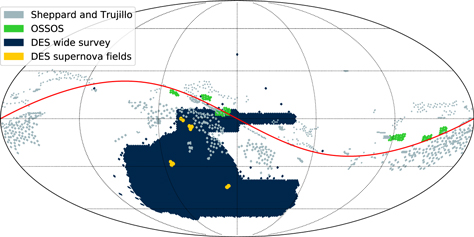
Figure 1. HEALPix mapping of the currently released sky coverage of the three major TNO surveys of this generation. The surveys by OSSOS and ST hug the ecliptic plane (plotted in red), while DES, designed as a cosmological survey, has a much more expansive footprint.
Download figure:
Standard image High-resolution imageThe most complete way to account for survey bias in the discovery of the solar system objects is to use a survey simulator (Petit et al. 2011; Lawler et al. 2018). In essence, a survey simulator simulates detections of a model population of solar system bodies by using a survey's pointing history, depth, and tracking criteria. This allows for the computation of a survey's selection function for a given population, which enables us to account for bias and therefore understand the true underlying populations. While it gives a reasonable approximation, the technique employed in BB19 cannot fully substitute for actually simulating each survey to calculate its selection function. Since the known ETNOs were discovered by a variety of surveys, the task of developing an appropriate simulator is nontrivial. Our simulator (FastSSim) is highly parametric, requiring only the few pieces of information common among all well-characterized surveys: pointing history, limiting magnitudes, and follow-up criteria. 46 The basic flow of the simulator is as follows:
- 1.
- 2.Generate a distribution of fake objects at a single epoch.
- 3.Calculate the objects’ HEALPix pixels and apparent magnitudes.
- 4.Determine which fake objects fall in a survey's footprint.
- 5.Make cuts according to the survey's limiting magnitudes and follow-up criteria.
Note that this simulation method makes several approximations. We compute the sky coordinates of our objects at a single epoch, we use a single color and limiting magnitude for each survey field, we do not consider CCD-level detections (so we do not account for complications such as chip gaps), and we employ a step-function detection criterion (so we do not model survey cadence or linking efficiency). We use a single HEALPix pixel for each survey pointing. We have chosen the pixel scales for each telescope as follows: Blanco uses an NSIDE of 64 (except for the DES supernova fields, for which we use an NSIDE of 1024), and the Magellan, Large Binocular, and Subaru telescopes use an NSIDE of 128. These assumptions ignore the time history of the surveys, as well as the apparent motion of the objects. FastSSim works well for this application because the objects move slowly, the telescopes have large fields of view, and the sensitivity does not have much spatial variation.
We acquired the non-DES survey pointings and limiting magnitudes from ST, Sheppard et al. (2019), and Bannister et al. (2018). We choose each HEALPix pixel size to most closely match the field of view of the telescope used. This does not allow for a perfect mapping between pointings and pixels, but it turns out to be sufficient for our needs. In fact, we find that FastSSim performs remarkably well in cross-checks against both our full chip-level DES simulator (Hamilton 2019) and the OSSOS survey simulator described in Petit et al. (2011; see Figure 2). While FastSSim misses some of the fine details of the selection functions, the small sample of ETNOs and the approximate nature of this analysis make such fine details unimportant to our overall conclusion. Given the success of these cross-checks, we are confident in extending their use to characterize the survey of ST.
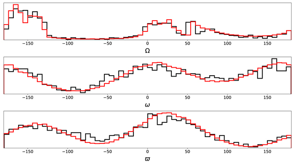
Figure 2. OSSOS selection functions for 1615 detections from the nominal population described in Section 3 in the angles ω, Ω, and ϖ, as calculated by FastSSim (red) and the OSSOS/CFEPS survey simulator (black). The distributions have the same general shape.
Download figure:
Standard image High-resolution imageTo simulate the surveys, we randomly generate ETNOs in accordance with a nominal scattered-disk model (specified in Section 3) until each survey has accumulated 105 detections, to allow for high-resolution characterization of a survey's sensitivity in ϖ and Ω. This typically requires the generation of approximately 1010 fakes, so our set of simulated objects spans the parameter space of the ETNOs. We consider an object to be detected if it is in one of the survey's HEALPix pixels, is brighter than the pixel's limiting magnitude, and has a perihelion distance q ≥ 30 au. For the survey of ST, we satisfy a tracking criterion specified in Sheppard et al. (2016) by requiring an object to have a heliocentric distance of at least 50 au at the time of detection.
As a quantitative example of the effectiveness of FastSSim, Figure 2 shows a comparison with the CFEPS/OSSOS simulator. For this test, each simulator uses the population model defined in Section 3. Using Kuiper's test, we find that the distributions of the 1615 data points calculated by FastSSim are statistically indistinguishable from those computed using the CFEPS/OSSOS survey simulator. Thus, in order to distinguish the two simulators, one would need >1,615 ETNOs—well above the quantity discovered by OSSOS. We achieve similar results in quantitative comparisons against the distributions computed using the DES survey simulators (see Figure 5.1 in Hamilton 2019 and Figure 2 in Bernardinelli et al. 2020a).
In Figure 3, we plot a Gaussian kernel density estimate of each simulator's detections in the (x, y) and (p, q) spaces (x, y, p, and q are defined in Section 4). Since the distributions appear to be in good agreement, we believe that our selection functions, which are derived directly from the surveys’ pointing histories, depths, and TNO tracking strategies, more faithfully model their respective surveys than those inferred indirectly in BB19 (see their Figure 4). Furthermore, the p-values we calculate using the CFEPS/OSSOS survey simulator do not significantly differ from those we calculate using FastSSim.
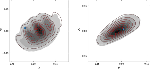
Figure 3. The black contours (which follow a linear scale) are Gaussian kernel density estimates of 106 iterations of sampling five points from the OSSOS biases calculated using the CFEPS/OSSOS survey simulator (because OSSOS discovered five ETNOs) and plotting the mean (x, y) and (p, q) positions (see Section 4 for definitions of x, y, p, and q). The red contours represent the same statistic, calculated using FastSSim. The blue points are the mean positions of the five ETNOs discovered by OSSOS. Our simulator reproduces the results of the OSSOS simulator with better fidelity than the heuristic method of BB19 (see their Figure 4).
Download figure:
Standard image High-resolution image3. Scattered-disk Model
To test the dependence of our analysis on the choice of scattered-disk model, we simulated models with various distributions of semimajor axis (a), eccentricity (e), inclination (i), and absolute magnitude (H) while keeping the orbital angles Ω and ω (and thus ϖ) uniform from 0° to 360°. We tested manifold permutations with the parameter distributions: N(a) ∝ aζ with a ∈ [230 au, 1600 au] and ζ ∈ [0.5, 1.0], uniform i ∈ [0°, 60°], Brown distribution i (Brown 2001) with a variety of widths ranging from 5° to 25°, and N(H) ∝ 10H ζ with H ∈ [4, 10] and ζ ∈ [0.6, 0.9].
We found that our conclusions were not significantly affected by the variation of the model parameters. Our results are also robust to changes in pericenter distribution (see the Appendix for the distribution of orbital elements for populations with q > 30, 35, and 38 au). Shankman et al. (2017) found a similar resilience to changes in the scattered-disk model. Noting the weak dependence of the outcome of our simulations on the choice of model, we proceed using the following scattered-disk model:
- 1.a follows a single power-law distribution such that N(a) ∝ a0.7, where a ∈ [230 au, 1600 au];
- 2.e is distributed uniformly ∈ [0.69, 0.999];
- 3.i follows a Brown distribution such that
![$N(i)\,\propto \sin (i)\exp \left[-\tfrac{{\left(i-{\mu }_{i}\right)}^{2}}{2{\sigma }_{i}^{2}}\right]$](https://content.cld.iop.org/journals/2632-3338/2/2/59/revision2/psjabe53eieqn1.gif) , with μi
= 0° and σi
= 15°;
, with μi
= 0° and σi
= 15°; - 4.H follows a single power-law distribution such that N(H) ∝ 100.8H , where H ∈ [4, 10]; and
- 5.the perihelion distance q > 30 au.
These model parameters produce posteriors in a, e, q, i, and H that appear to be in reasonable agreement with the real ETNO detections by each survey. See the Appendix for histograms of the posteriors in each of these variables, overlaid with a rug plot of each survey's real detections.
4. Analysis and Results
Performing a clustering analysis in the variables ϖ and Ω is complicated, as the two are strongly correlated. We proceed by working in the orthogonal {x, y, p, q} basis discussed in BB19 (importantly, ϖ and Ω are linearly independent in this basis). Note that these vectors are not normalized but instead have their lengths modulated by eccentricity and inclination. The coordinates are defined as follows:



Note that Γ and Z have been scaled by a factor of  from their traditional forms, since the semimajor axis is not relevant to this argument. Figure 4 shows our calculated selection functions in the xy- and pq-planes.
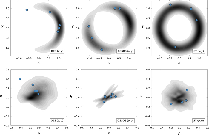
Figure 4. Kernel density estimates of each survey's selection function in the canonical xy-space (top row) and pq-space (bottom row). The contours represent simulated detections (the contours scale linearly, and darker contours are more densely populated), while the blue dots represent the ETNOs detected by each survey. The outlier in both DES panels is the object 2015 BP519 (Becker et al. 2018).
Download figure:
Standard image High-resolution imageFor the sake of comparison, we used the method presented in BB19 to test the consistency of each survey's detected ETNOs with its selection function. We first perform 106 iterations, sampling from our simulated detections a set of objects whose cardinality is equal to that of the set of real ETNOs detected by the given survey. We then take the average {x, y, p, q} position of each sample and use these values to construct a four-dimensional histogram. We display a Gaussian kernel density estimation of these data in the xy- and pq-planes in Figure 5.
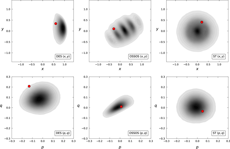
Figure 5. Kernel density estimates of the mean (x, y) and (p, q) position of 106 samples of ETNOs drawn from the PDFs shown in Figure 4. The number of objects in each sample corresponds to the number of ETNOs detected by the given survey. The contours represent the samples (the contours scale linearly, and darker contours are more densely populated), while the red dots represent the mean position of the ETNOs detected by each survey.
Download figure:
Standard image High-resolution imageWe perform a Gaussian kernel density estimation on our mean-sampled histograms to obtain a probability distribution function (PDF). Next, we draw N samples from our simulated data (where N is the number of ETNOs actually detected by the survey), find the mean {x, y, p, q} position, and evaluate our PDF at that position. We repeat this 105 times to construct a likelihood function. Next, we compute this value for the ETNOs actually discovered by the survey. To calculate the probability of a survey detecting the ETNOs it actually detected (as opposed to some other set of ETNOs), we find the fraction of the 105 sample likelihood values that the survey's actual likelihood value exceeds. Rounded to the nearest 1%, this probability for each survey is as follows:  ,
,  , and
, and  .
.
The joint probability of N surveys detecting objects with given probabilities (or some less likely set of values) can be calculated as the volume under the surface of a constant product of probabilities in the domain of the N-dimensional unit hypercube, given by

where  . In our case, k ∈ {DES, OSSOS, ST}. Using Equation (4), we calculate the joint probability to be 24%.
With such a small sample size, this work is sensitive to outliers and the definition of “ETNO” itself. The high-inclination object 2015 BP519 is among the most dynamically anomalous objects in the solar system (Becker et al. 2018), and we cannot discount the possibility that it is of a different dynamical origin than the other ETNOs. If we redo our analysis without 2015 BP519,  increases to 84%, and thus
  increases to ∼ 85%. The object 2014 FE72 has an extremely large semimajor axis—roughly four standard deviations above the mean of the ETNOs considered in this work. Its large semimajor axis carries it deep into the IOC region, where interactions with galactic tides make its secular relationship with a putative Planet X/Planet 9 less certain. If we exclude 2014 FE72,
  increases to 88%, and thus
  increases to 31%. If we include 2012 VP113,
  increases to 60%, and
  remains 24%. We also address the fact that the clustering by a putative Planet X/Planet 9 should be more robust in the sample of ETNOs with q > 40 au, since these objects avoid strong perturbations by Neptune. If we restrict our ETNOs to these eight objects,
  increases to 94%. Finally, we analyze the subset of objects that are either stable or metastable in the presence of the putative Planet X/Planet 9 (Batygin et al. 2019): 2015 TG387, 2013 SY99, 2015 RX245, 2014 SR349, 2012 VP113, 2013 RA109, and 2013 FT28. For this subset,
  .
.
For the sake of completeness, we also use a more traditional sampling method to determine the significance of the clustering of ETNOs. We begin by performing a Gaussian kernel density estimate on each survey's posterior distributions. We then perform 105 iterations in which we randomly draw N points from each survey's posterior distribution (where N is the number of ETNOs detected by the survey) and multiply each of the N probabilities together to calculate a likelihood. Finally, we calculate the same metric for each survey's actual detections and compare the value to the distribution of our samples. As before, the probability for each survey is the fraction of the 105 sample likelihood values that the survey's actual likelihood value exceeds. Rounded to the nearest 1%, the probability for each survey is as follows:  ,
,  , and
, and  . The joint probability is thus 17%.
For a more physically intuitive representation of the survey bias, refer to Figure 6. Here the radial quantity represents the barycentric distance, and the azimuthal quantity represents true longitude (the true anomaly + ϖ). The edge of the black circle is at 30 au. The white regions represent the combined surveys’ sensitivity (brighter regions correspond to higher sensitivity), weighted by the number of real ETNO detections. The red dots represent the real ETNOs at the epoch of discovery. The observations are in good agreement with the combined selection function, qualitatively confirming the conclusions of our formal statistical analysis performed on canonical variables.
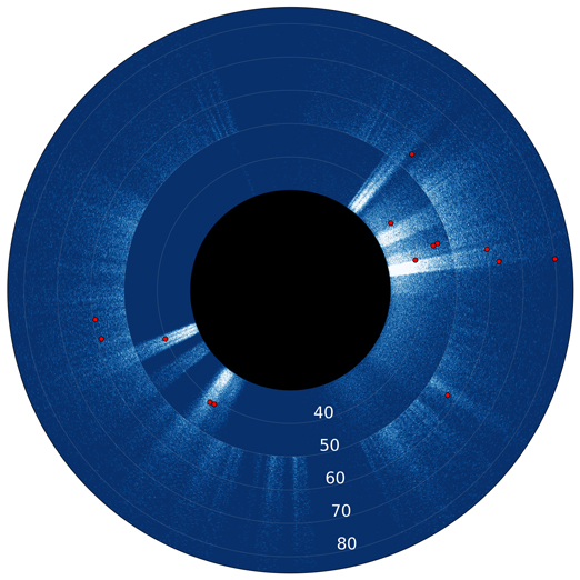
Figure 6. Combined ETNO selection function for all three surveys. The radial quantity is the ETNO's barycentric distance, and the azimuthal quantity is true longitude. The edge of the black circle is at 30 au. The white regions represent the combined surveys’ sensitivity (brighter regions correspond to higher sensitivity), weighted by the number of real ETNO detections. The red dots represent the real ETNOs at the epoch of discovery. The outer ring is caused by the 50 au tracking criterion imposed by ST.
Download figure:
Standard image High-resolution image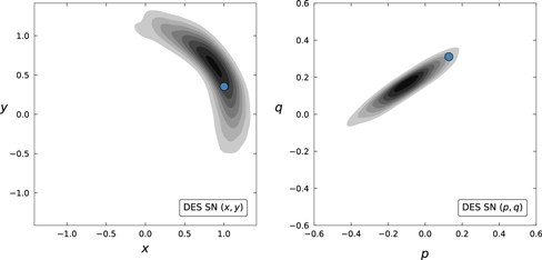
Figure 7. Kernel density estimates of the DES SN selection function in the canonical xy-space (left) and pq-space (right). The contours represent simulated detections (the contours scale linearly, and darker contours are more densely populated), while the blue dots represent 2013 RF98.
Download figure:
Standard image High-resolution image4.1. DES Supernova Fields
The ETNO 2013 RF98 was discovered in the deep DES supernova (DES SN) fields. Since the DES SN fields are so small, they suffer from severe selection bias. Additionally, since their observing cadence and depth (∼24.5 in the r band) are significantly different from those of the wide survey, they need to be treated independently. We generated 1829 simulated detections in the DES SN fields (since the fields are so small, it is computationally prohibitive to generate 105 synthetic detections, as we do for DES, OSSOS, and ST) from the population model defined in Section 3. Figure 7 shows a kernel density estimate of the detections in {x, y, p, q} space. We show the posteriors in {a, e, i, H, Ω, ϖ} in Figures 8–14 in the Appendix. In all parameters, 2013 RF98 appears to be a rather ordinary detection for the DES SN fields.
Since there is only one data point here, we can just numerically integrate to find  (i.e., a p-value of 0.33). Treating DES SN as its own survey, we may use Equation (4) to calculate the four-survey joint probability to find
  .
.
5. Discussion and Conclusions
We use quantified selection bias calculations on all ETNOs discovered by the three most productive ETNO surveys, each with a quite different survey strategy and selection function, to test the consistency of the ETNOs with a uniform underlying distribution. Given a joint probability between 17% and 94% (i.e., a p-value between 0.17 and 0.94), we conclude that the sample of ETNOs from well-characterized surveys is fully consistent with an underlying parent population with uniform distributions in the longitudes ϖ and Ω. Our result differs drastically from the corresponding value in BB19 of 0.2%. Closer inspection sheds some light on the apparent discrepancy. If we examine only the overlapping set of ETNOs used this work and BB19 (2015 BP519, 2013 RF98, 2013 SY99, 2015 RX245, 2015 GT50, 2015 KG163, 2013 FT28, 2014 SR349, and 2014 FE72),  drops to <0.005. This indicates an expected issue: small number statistics are sensitive to fluctuations. For example, when BB19 performed their analysis, a small but important set of ETNOs had not yet been reported to the MPC. As a concrete demonstration of the importance of the omission of a few ETNOs from BB19, consider DES. Of the five ETNOs discovered by the DES wide survey, BB19 included only 2015 BP519. From Figure 4, it is clear that this object lands in an extremely low-probability region. This drives down
  and thus gives a satisfactory answer as to why the result of this work differs so significantly from that of BB19.
It is important to note that our work does not explicitly rule out Planet X/Planet 9; its dynamical effects are not yet well enough defined to falsify its existence with current data. This work also does not analyze whether some form of clustering could be consistent with the 14 ETNOs we consider. For example, the ETNOs could happen to be clustered precisely where current surveys have looked. In that case, a survey with coverage orthogonal to the regions shown in Figure 6 would find far fewer ETNOs than expected. Various realizations of Planet X/Planet 9 predict clustering of various widths, modalities, and libration amplitudes and frequencies; we do not test for consistency with any of these distributions. Instead, we have shown that, given the current set of ETNOs from well-characterized surveys, there is no evidence to rule out the null hypothesis. Increasing the sample of ETNOs with ongoing and future surveys with different selection functions, such as the Deep Ecliptic Exploration Project (Trilling et al. 2019) and the Legacy Survey of Space and Time at the Vera Rubin Observatory (Schwamb et al. 2018), will allow for more restrictive results. Despite other lines of indirect evidence for Planet X/Planet 9, in the absence of clear evidence for clustering of the ETNOs, the argument becomes much weaker. Future studies should consider other mechanisms capable of giving the outer solar system its observed structure while preserving a uniform distribution of ETNOs in the longitudes Ω and ϖ.
This material is based upon work supported by the National Aeronautics and Space Administration under grant No. NNX17AF21G issued through the SSO Planetary Astronomy Program and by the National Science Foundation under grant No. AST-2009096.
Funding for the DES Projects has been provided by the U.S. Department of Energy, the U.S. National Science Foundation, the Ministry of Science and Education of Spain, the Science and Technology Facilities Council of the United Kingdom, the Higher Education Funding Council for England, the National Center for Supercomputing Applications at the University of Illinois at Urbana-Champaign, the Kavli Institute of Cosmological Physics at the University of Chicago, the Center for Cosmology and Astro-Particle Physics at the Ohio State University, the Mitchell Institute for Fundamental Physics and Astronomy at Texas A&M University, Financiadora de Estudos e Projetos, Fundação Carlos Chagas Filho de Amparo à Pesquisa do Estado do Rio de Janeiro, Conselho Nacional de Desenvolvimento Científico e Tecnológico and the Ministério da Ciência, Tecnologia e Inovação, the Deutsche Forschungsgemeinschaft, and the Collaborating Institutions in the Dark Energy Survey.
The Collaborating Institutions are Argonne National Laboratory, the University of California at Santa Cruz, the University of Cambridge, Centro de Investigaciones Energéticas, Medioambientales y Tecnológicas-Madrid, the University of Chicago, University College London, the DES-Brazil Consortium, the University of Edinburgh, the Eidgenössische Technische Hochschule (ETH) Zürich, Fermi National Accelerator Laboratory, the University of Illinois at Urbana-Champaign, the Institut de Ciències de l’Espai (IEEC/CSIC), the Institut de Física d’Altes Energies, Lawrence Berkeley National Laboratory, the Ludwig-Maximilians Universität München and the associated Excellence Cluster Universe, the University of Michigan, NFS's NOIRLab, the University of Nottingham, The Ohio State University, the University of Pennsylvania, the University of Portsmouth, SLAC National Accelerator Laboratory, Stanford University, the University of Sussex, Texas A&M University, and the OzDES Membership Consortium.
Based in part on observations at Cerro Tololo Inter-American Observatory at NSF's NOIRLab (NOIRLab Prop. ID 2012B-0001; PI: J. Frieman), which is managed by the Association of Universities for Research in Astronomy (AURA) under a cooperative agreement with the National Science Foundation.
The DES data management system is supported by the National Science Foundation under grant Nos. AST-1138766 and AST-1536171. The DES participants from Spanish institutions are partially supported by MICINN under grants ESP2017-89838, PGC2018-094773, PGC2018-102021, SEV-2016-0588, SEV-2016-0597, and MDM-2015-0509, some of which include ERDF funds from the European Union. The IFAE is partially funded by the CERCA program of the Generalitat de Catalunya. Research leading to these results has received funding from the European Research Council under the European Union's Seventh Framework Program (FP7/2007-2013), including ERC grant agreements 240672, 291329, and 306478. We acknowledge support from the Brazilian Instituto Nacional de Ciência e Tecnologia (INCT) do e-Universo (CNPq grant 465376/2014-2).
This manuscript has been authored by the Fermi Research Alliance, LLC, under contract No. DE-AC02-07CH11359 with the U.S. Department of Energy, Office of Science, Office of High Energy Physics.
Appendix
In Figures 8–14 we show the posterior distributions of the orbital elements of our simulated detections.
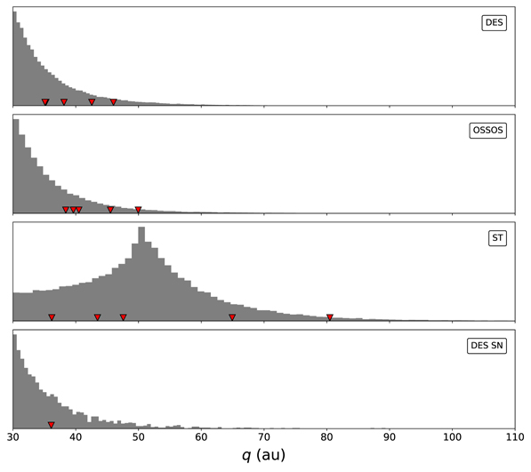
Figure 8. Posterior pericenter distance distributions of simulated detections. The red triangles are the real ETNO detections by each survey. Note that DES has partially overlapping data points at q ≈ 35 au.
Download figure:
Standard image High-resolution image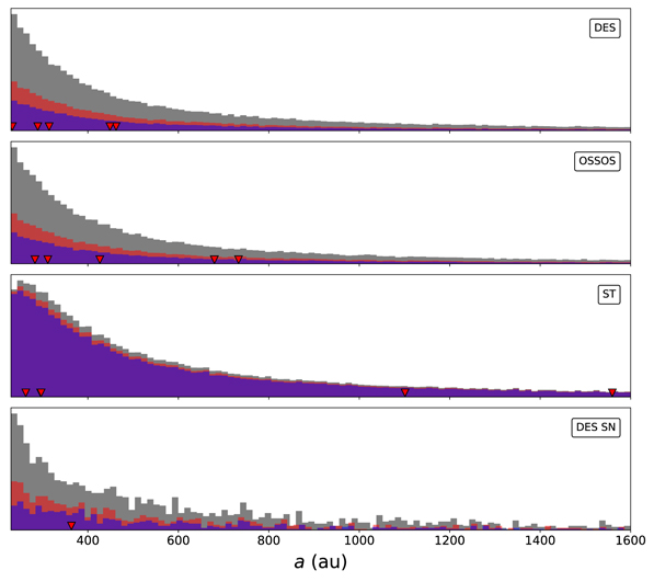
Figure 9. Posterior semimajor axis distributions of simulated detections. The red triangles are the real ETNO detections by each survey. Note that ST has partially overlapping data points at a ≈ 296 au. The gray, red, and blue histograms correspond to cuts with q > 30, 35, and 38 au, respectively.
Download figure:
Standard image High-resolution image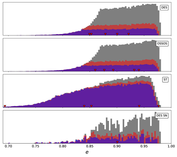
Figure 10. Posterior eccentricity distributions of simulated detections. The red triangles are the real ETNO detections by each survey. Note that DES has overlapping data points at e = 0.85. The gray, red, and blue histograms correspond to cuts with q > 30, 35, and 38 au, respectively.
Download figure:
Standard image High-resolution image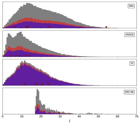
Figure 11. Posterior inclination distributions of simulated detections. The red triangles represent the real ETNO detections by each survey. The gray, red, and blue histograms correspond to cuts with q > 30, 35, and 38 au, respectively.
Download figure:
Standard image High-resolution image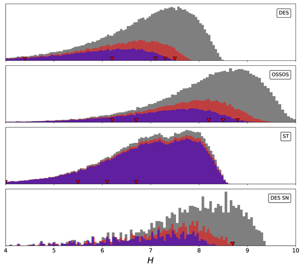
Figure 12. Posterior absolute magnitude distributions of simulated detections. The red triangles represent the real ETNO detections by each survey. Note that ST has overlapping data points at H = 6.7. The gray, red, and blue histograms correspond to cuts with q > 30, 35, and 38 au, respectively.
Download figure:
Standard image High-resolution image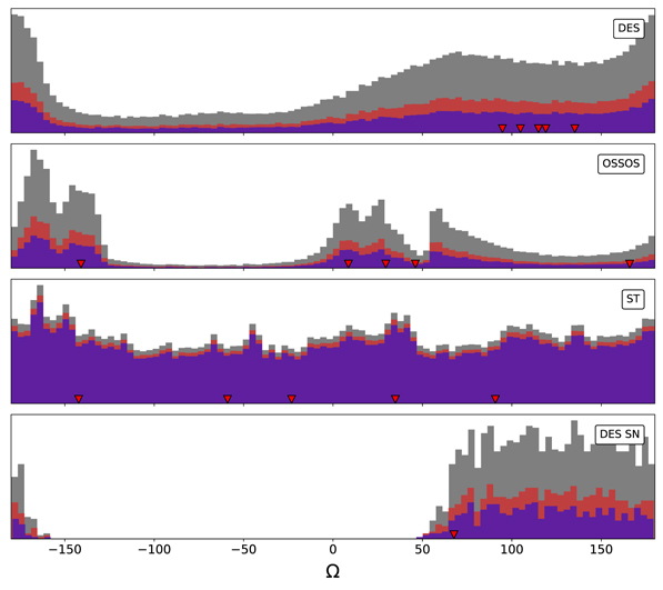
Figure 13. Posterior longitude of ascending node distributions of simulated detections. The red triangles represent the real ETNO detections by each survey. The gray, red, and blue histograms correspond to cuts with q > 30, 35, and 38 au, respectively.
Download figure:
Standard image High-resolution image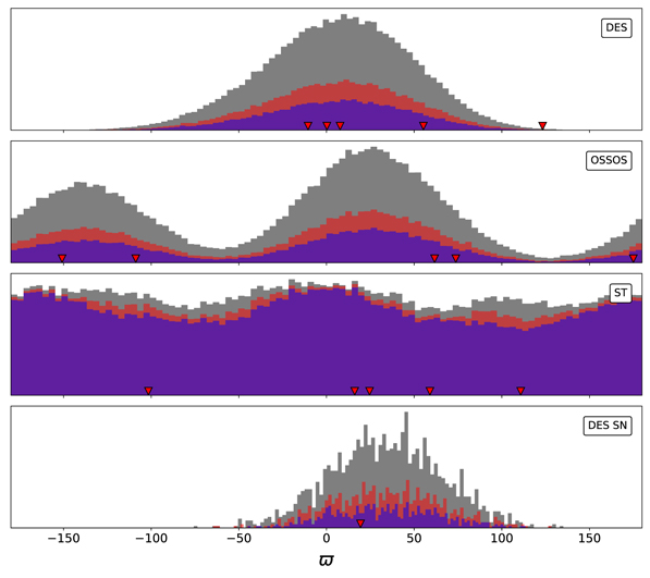


Figure 14. Posterior longitude of pericenter distributions of simulated detections. The red triangles represent the real ETNO detections by each survey. The gray, red, and blue histograms correspond to cuts with q > 30, 35, and 38 au, respectively.
Download figure:
Standard image High-resolution image

Footnotes
- 46
The tools for the FastSSim algorithm have now been compiled into the open-source Python package SpaceRocks. It is under active development at https://github.com/kjnapier/spacerocks.
- 47
It is not important that we used a HEALPix mapping. We could have used any mapping onto the sphere.