

ABSTRACT
Much of the dynamical structure of the Kuiper Belt can be explained if Neptune migrated over several AU, and/or if Neptune was scattered to an eccentric orbit during planetary instability. An outstanding problem with the existing formation models is that the distribution of orbital inclinations they predicted is narrower than the one inferred from observations. Here we perform numerical simulations of Kuiper Belt formation starting from an initial state with Neptune at  AU and a dynamically cold outer disk extending from beyond
  to 30 AU. Neptune’s orbit is migrated into the disk on an e-folding timescale 1 ≤ τ ≤ 100 Myr. A small fraction (∼10−3) of the disk planetesimals become implanted into the Kuiper belt in the simulations. By analyzing the orbital distribution of the implanted bodies in different cases we find that the inclination constraint implies that
  Myr and
  AU. The models with
  Myr do not satisfy the inclination constraint, because there is not enough time for various dynamical processes to raise inclinations. The slow migration of Neptune is consistent with other Kuiper Belt constraints, and with recently developed models of planetary instability/migration. Neptune’s eccentricity and inclination are never large in these models (
 ,
,  ), as required to avoid excessive orbital excitation in the >40 AU region, where the Cold Classicals presumably formed.
1. BACKGROUND
The Kuiper Belt is a diverse population of trans-Neptunian bodies (Figure 1). Based on dynamical considerations, the Kuiper Belt Objects (KBOs) are classified into several groups: the resonant populations, classical belt, scattered/scattering disk, and detached objects (also known as the fossilized scattered disk). See Gladman et al. (2008) for a formal definition of these groups. The resonant populations are a fascinating feature of the Kuiper Belt. They give the Kuiper Belt an appearance of a bar code with individual bars centered at the resonant orbital periods. While Pluto and Plutinos in the 3:2 resonance with Neptune (orbital period  years) are the largest and the best-characterized resonant group, nearly every resonance hosts a large population of bodies. The resonant bodies are long-lived, because they are phase-protected by the resonance from close encounters with Neptune. The orbits of the scattered/scattering disk objects, on the other hand, evolved and keep evolving by close encounters with Neptune. These objects tend to have long orbital periods and to be detected near their orbital perihelion when the heliocentric distance is ∼30 AU. Their neighbors, the detached objects, have a slightly larger perihelion distance than the scattered/scattering objects and semimajor axes beyond the 2:1 resonance (
 AU). The detached objects probably suffered close encounters with Neptune in the past, were scattered to orbits with large semimajor axes and eccentricities (
 defines them in Gladman et al. 2008), but then they became “detached” from Neptune when some process increased their perihelion distance (or when Neptune’s orbit circularized; Levison et al. 2008).
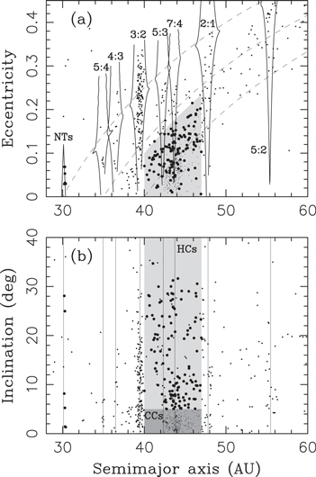
Figure 1. The orbital elements of KBOs observed in three or more oppositions. Various dynamical classes are highlighted. The HCs with  and NTs are denoted by larger dots, and the CCs are denoted by smaller dots. Note the wide inclination distribution of the HCs in panel (b) with inclinations reaching above
  . The solid lines in panel (a) follow the borders of important mean motion resonances. For the NTs, we show the approximate location of stable librations from Nesvorný & Dones (2002). The low-inclination orbits with
  AU are unstable due to secular resonance overlap (
 and
and  ; Kněžević et al. 1991; Duncan et al. 1995).
Download figure:
Standard image High-resolution imageThe classical belt is a population of trans-Neptunian bodies dynamically defined as having non-resonant orbits with perihelion distances that are large enough to avoid close encounters with Neptune. They can be thought of as being related to the detached objects but having orbits with modest orbital eccentricities ( according to Gladman et al. 2008). Here we consider the main classical belt located between the 3:2 and 2:1 resonances with Neptune (
 AU), because this is where most known classical objects reside. It is useful to divide the main belt into the dynamically “cold” and “hot” components, mainly because the inclination distribution of the main belt orbits is bimodal (Brown 2001), hinting at different dynamical origins for these components. Here we adopt an approximate separation, with Cold Classicals (CCs) being defined as having
  and Hot Classicals (HCs) as
  . Note that this definition is somewhat arbitrary, because the continuous inclination distribution near
  indicates that mixing between the two components must have happened (e.g., Morbidelli et al. 2008; Volk & Malhotra 2011).
While the HCs share many similarities with other dynamical classes of KBOs (e.g., scattered disk, Plutinos), the CCs have several unique properties. Specifically, (1) the CCs have distinctly red colors (e.g., Tegler & Romanishin 2000) that may have resulted from space weathering of surface ices, such as ammonia (Brown et al. 2011), that are stable beyond ∼35 AU. (2) A large fraction of the 100 km-class CCs are wide binaries with nearly equal size components (Noll et al. 2008a, 2008b). (3) The albedos of the CCs are generally higher than those of the HCs (Brucker et al. 2009). And finally, (4) the size distribution of the CCs is markedly different from those of the hot and scattered populations, in that it shows a very steep slope at large sizes (e.g., Bernstein et al. 2004; Fraser et al. 2014), and lacks very large objects (Levison & Stern 2001). The most straightforward interpretation of these properties is that the CCs formed and/or dynamically evolved by different processes than other trans-Neptunian populations.
Following the pioneering work of Malhotra (1993, 1995), studies of Kuiper Belt dynamics first considered the effects of outward migration of Neptune that can explain the prominent populations of KBOs in major resonances (Hahn & Malhotra 1999, 2005; Chiang & Jordan 2002; Chiang et al. 2003; Gomes 2003; Levison & Morbidelli 2003; Murray-Clay & Chiang 2005, 2006). With the advent of the notion that the early solar system may have suffered a dynamical instability (Thommes et al. 1999; Tsiganis et al. 2005), the focus broadened, with the more recent theories invoking a transient phase with an eccentric orbit of Neptune (Levison et al. 2008; Morbidelli et al. 2008; Batygin et al. 2011; Wolff et al. 2012).
The emerging consensus is that the HCs, together with the resonant, scattered, and detached populations, formed in a massive planetesimal disk at  AU, and were dynamically scattered onto their current orbits by migrating (and possibly eccentric) Neptune, while the CCs formed at >40 AU and survived Neptune’s early “wild days” relatively unharmed (Batygin et al. 2011; Wolff et al. 2012). The main support for this model comes from the unique properties of the CCs, which would be difficult to explain if the HCs and CCs had similar formation locations (and dynamical histories). For example, the wide binaries observed among the CCs would not survive scattering encounters with Neptune (Parker & Kavelaars 2010). Moreover, if the CCs evolved from the high-eccentricity Neptune-crossing orbits, this process should produce a gradient in e with more orbits having large e and fewer orbits having small e. The CCs do not show such a trend. Instead, low eccentricities prevail in that population.
2. THE INCLINATION PROBLEM
The inclination distribution of various populations in the Kuiper Belt can be represented by  , where
  is a parameter (Brown 2001). In the main belt, the inclination distribution is bimodal and two components are needed:
  for the low-i CCs and
  −17° for the high-i HCs (Brown 2001; Kavelaars et al. 2008, 2009). The low inclinations of CCs are in line with the expectation that they formed from a dynamically cold disk at >40 AU, and their orbits were never excited too much by subsequent dynamical processes. The high inclinations of the HCs, on the other hand, are more challenging to explain (see below). Moreover, there is some evidence from high-latitude surveys that
  may be somewhat inadequate, because the drop-off at large values of i is probably steeper than expected from this functional dependence (Petit et al. 2015). For this reason, it is possible that
  with
with  may better represent the underlying distribution.
The HC distribution with relatively high orbital inclinations is shared among several other Kuiper Belt populations as well, including Neptune Trojans (NTs), and the resonant and scattered objects. Eight NTs are currently known. Four of them have orbital inclinations  , and four have
  . This could mean that the distribution is bimodal, but Parker (2015) showed that the bimodality of the underlying inclination distribution cannot be demonstrated with confidence from the existing data. If the distribution is parametrized by a single term,
  , the NTs are inferred to have
  with a 95% confidence (Parker 2015). Plutinos in the 3:2 resonance with Neptune are well represented by a single term with
  according to Gulbis et al. (2010), or
  according to Kavelaars et al. (2008, p. 59) and Gladman et al. (2012). Interestingly, the CC-like component with low orbital inclinations is not found in the Plutino population.
The wide inclination distribution of the HCs, NTs, Plutinos, and other resonant populations poses an important constraint on dynamical models of Kuiper Belt formation.1
It implies that some dynamical process must have increased the inclinations by 10°–15° on average, and by ≃30° at least in some cases. For example, the inclination constraint can be used to rule out a model in which these populations arise from a dynamically cold planetesimal disk at >30 AU, simply because the orbital inclinations are not excited in this region during Neptune’s migration (passing mean motion resonances do not affect inclinations much). Hahn & Malhotra (2005) investigated this issue in detail and found that starting with moderately excited orbits of planetesimals (e.g.,  ) does not resolve the problem, because the final inclination distribution is still not wide enough.2
The only way to make things work in the context of the Hahn & Malhotra model would be to assume that the inclinations were already high before Neptune’s migration, but that seems unsatisfactory, because it is not clear how the inclinations could have been excited beforehand. Lykawka & Mukai (2008) considered dynamical effects of an additional planet in the trans-Neptunian region. They found that this putative planet could help to excite inclinations, but the inclination distribution obtained in their model was not wide enough to match observations well. It lacked orbits in the classical belt with
) does not resolve the problem, because the final inclination distribution is still not wide enough.2
The only way to make things work in the context of the Hahn & Malhotra model would be to assume that the inclinations were already high before Neptune’s migration, but that seems unsatisfactory, because it is not clear how the inclinations could have been excited beforehand. Lykawka & Mukai (2008) considered dynamical effects of an additional planet in the trans-Neptunian region. They found that this putative planet could help to excite inclinations, but the inclination distribution obtained in their model was not wide enough to match observations well. It lacked orbits in the classical belt with  , while these orbits are in fact common.
Given the difficulties described above, various theoretical models considered the formation of the HCs and resonant populations from a massive planetesimal disk at <30 AU. The outer edge of the massive disk is constrained to  AU by Neptune’s present orbit (Gomes et al. 2004). The disk could have been truncated, for example, by photoevaporation or a close stellar encounter (e.g., Adams 2010; Kretke et al. 2012). To reach >40 AU, planetesimals must be radially displaced. Levison & Morbidelli (2003) considered a scenario in which objects were pushed out by the 2:1 resonance with Neptune. This could work only if Neptune was initially inside
  AU, such that the 2:1 resonance fell inside the massive disk’s outer boundary at
  AU. Gomes (2003), on the other hand, suggested that bodies were first scattered to >40 AU by having close encounters with Neptune, and became dynamically decoupled from Neptune while Neptune was still migrating. If so, the HCs and resonant populations would be close relatives of the scattered disk objects. The exact nature of the decoupling process for the HCs is uncertain (Gomes 2003; Levison et al. 2008; Dawson & Murray-Clay 2012), but recent work suggests that capture into mean motion resonances with Neptune (2:1, 5:3, 7:4, etc.), and secular/Kozai cycles inside the resonances may have played an important role (Brasil et al. 2014b).
These results could help to resolve the inclination problem discussed above, because the orbital inclinations can be excited when bodies undergo a series of close encounters with Neptune (Gomes 2003). In addition, inclinations are increased for orbits that suffer Kozai cycles, because to decouple from Neptune, the eccentricity must drop, and the inclination would therefore rise (due to the anticorrelated behavior of e and i caused by the Kozai cycles; Kozai 1962). It remains to be shown, however, how these processes operated to affect the Kuiper Belt, and how the early evolution of planetary orbits is constrained by the dynamical structure of the Kuiper Belt.
As demonstrated in Figure 2, the inclination problem is not resolved by simply postulating that much of the Kuiper Belt has been implanted from <30 AU (e.g., see discussion in Petit et al. 2011). Here we choose to illustrate the inclination problem with Plutinos, because the 3:2 resonance population is characterized much better than any other resonant population (e.g., Gladman et al. 2012). Also, Plutinos do not show the bimodal inclination distribution of the classical belt, so we do not need to worry about the overlap of different groups. The parameters of the numerical model from Figure 2 are similar to those used in Levison et al. (2008). We used a fast migration regime with an exponential e-folding timescale  Myr (see next section for our model description) to illustrate that such a fast migration of Neptune leads to an implausible result. There is simply not enough time in this case to substantially raise the orbital inclinations.
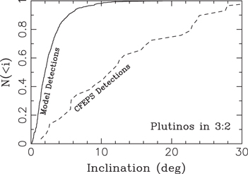
Figure 2. The cumulative inclination distribution of Plutinos in the 3:2 resonance with Neptune. The distribution of 29 Plutinos detected by CFEPS (dashed line, Petit et al. 2011) is compared to a model distribution (solid line). The K–S test applied to these distributions shows that the likelihood that they can be obtained from the same underlying distribution is 2 × 10⁻¹³. This rules out the model. The model distribution is a result of a numerical simulation where we considered Neptune’s migration into a dynamically cold disk ( and
and  ) at
) at  AU. See Section 3 for a description of the model. Here we used
  AU,
AU,  , and
, and  . The radial migration and eccentricity damping were applied to Neptune’s orbit on an e-folding timescale
  Myr. To compare apples with apples, the CFEPS simulator (see Section 4) was used to compute the detection statistics from the population of bodies that survived in the 3:2 resonance at the end of the simulation. Thus, both distributions shown in this plot include the observational bias of CFEPS. The inclination distribution obtained for larger values of
  (Levison et al. 2008 used
  ) is similar to the one shown here for
  .
.
Download figure:
Standard image High-resolution imageHere we perform numerical simulations to investigate the inclination problem in detail. Our method and constraints are described in Sections 3 and 4, and the results are presented in Section 5. We find that bodies starting with  AU can be implanted into the Kuiper Belt by first being scattered by Neptune to
  AU, and then decoupling from Neptune by various resonant effects while Neptune is still migrating (see Section 5.2). We show that the inclination constraint implies a prolonged phase during which Neptune slowly migrated (e-folding migration timescale
  Myr) before reaching its current orbit at a = 30.1 AU.3
The main effect of slow migration is that orbits are allowed to decouple from Neptune relatively late during the migration process. Consequently, Neptune is given more time to act, via scattering encounters, on the source population, thus increasing the orbital inclinations of bodies before they are implanted into the Kuiper Belt. The model with Neptune’s slow migration is also consistent with other Kuiper Belt constraints (Section 5). Various implications of this result are discussed in Section 6.
Myr) before reaching its current orbit at a = 30.1 AU.3
The main effect of slow migration is that orbits are allowed to decouple from Neptune relatively late during the migration process. Consequently, Neptune is given more time to act, via scattering encounters, on the source population, thus increasing the orbital inclinations of bodies before they are implanted into the Kuiper Belt. The model with Neptune’s slow migration is also consistent with other Kuiper Belt constraints (Section 5). Various implications of this result are discussed in Section 6.
3. THE INTEGRATION METHOD
Our numerical integrations track the orbits of four planets (Jupiter to Neptune) and a large number of test particles representing the outer planetesimal disk. To set up an integration, Jupiter, Saturn, and Uranus were placed on their current orbits. The dependence of the results on the orbital behavior of Jupiter, Saturn, and Uranus was found to be minor. We determined this by comparing our nominal results with fixed orbits to those obtained when these planets were forced to radially migrate. Neptune was placed on an orbit with semimajor axis  , eccentricity
  , and inclination
  . To cover the parameter space, we set
  , 24, 26, or 28 AU,
  , 0.1, or 0.3, and
  or 5°. We tested many different combinations of these parameters to understand their role in Kuiper Belt formation. The cases with
  AU or 24 AU,
  and
and  are a good proxy for the initial conditions of Hahn & Malhotra (2005), who studied a long-range migration of Neptune, and for the instability/migration models developed in Nesvorný & Morbidelli (2012). The case with
  AU and
  is similar to runs A, B, and C in Levison et al. (2008), whose choice was motivated by the strong planetary instability occurring in the Nice model (Tsiganis et al. 2005; Morbidelli et al. 2007). The cases with
  were favored by Dawson & Murray-Clay (2012) from the CC-related constraints.
The swift_rmvs4 code (Levison & Duncan 1994) was used to follow the evolution of planets and disk particles. The swift_rmvs4 code was modified to include fictitious forces that mimic Neptune’s radial migration and damping. These forces were parametrized by exponential e-folding timescales  ,
,  , and
, and  , where
  controls the radial migration rate, and
  and
and  control the damping rates of e and i. Here we set
 , because such roughly comparable timescales were suggested by previous work. Specifically, we used
  , 3, 10, 30, and 100 Myr, where
  Myr corresponds to the case considered by Levison et al. (2008), while
  Myr is preferred from the instability simulations of Nesvorný & Morbidelli (2012). By finetuning the migration parameters, the final semimajor axis of Neptune was set to be within 0.05 AU of its current mean
  AU, and the orbital period ratio,
  , where
  and
and  are the orbital periods of Neptune and Uranus, was adjusted to end up within 0.5% of its current value (
 ).
).
Each simulation included one million disk particles distributed from just outside Neptune’s initial orbit to 30 AU. Their radial profile was set such that the disk surface density  , where r is the heliocentric distance. The large number of disk particles was needed because the capture probability in different parts of the Kuiper Belt is expected to be ∼10−3−10−4. With 106 disk particles initially, this yields ∼100–1000 captured particles, and allows us to perform a detailed comparison of the model results with observations (Section 4). The disk particles were assumed to be massless such that their gravity does not interfere with the migration/damping routines. This means that the precession frequencies of planets are not affected by the disk in our simulations, while in reality they were. This is an important approximation, because the orbital precession of Neptune during its high-eccentricity phase can influence the degree of secular excitation of the CCs (Batygin et al. 2011).
All simulations were run to 1 Gyr. The interesting cases were extended to 4 Gyr with the standard swift_rmvs4 code (i.e., without migration/damping in the 1–4 Gyr interval). We performed 18 simulations in total. Three of these runs were designed to test the reproducibility of the results. While the results concerning the orbital distribution of bodies implanted into the Kuiper Belt (Sections 5.1–5.3) were found to be strictly reproducible, the efficiency of capture in the Kuiper Belt can vary by a factor of a few depending on the behavior of Neptune’s eccentricity during the simulation (see discussion in Section 5.4).
An additional uncertain parameter concerns the dynamical structure of the original planetesimal disk. It is typically assumed that the disk was dynamically cold with orbital eccentricities  and orbital inclinations
  . Some dynamical excitation could have been supplied by scattering off of Pluto-sized and larger objects that presumably formed in the disk (Stern & Colwell 1997; Kenyon et al. 2008).4
The magnitude of the initial excitation is uncertain, because it depends on several unknown parameters (e.g., the number of massive objects in the disk). Here we operate under the assumption that the orbital inclinations of disk particles were relatively small initially, and were excited during the main stage of planetary instability/migration, when bodies were implanted into the Kuiper Belt. This is a reasonable assumption, given that the notion of planetary instability/migration was developed, among other reasons, to explain the complex orbital structure of the Kuiper Belt. It would thus seem unsatisfactory to “resolve” the inclination problem discussed in Section 2 by postulating that the inclinations were already large initially (unless it is explained how that happened). The initial eccentricities and initial inclinations of disk particles in our standard simulations were distributed according to the Rayleigh distribution with
. Some dynamical excitation could have been supplied by scattering off of Pluto-sized and larger objects that presumably formed in the disk (Stern & Colwell 1997; Kenyon et al. 2008).4
The magnitude of the initial excitation is uncertain, because it depends on several unknown parameters (e.g., the number of massive objects in the disk). Here we operate under the assumption that the orbital inclinations of disk particles were relatively small initially, and were excited during the main stage of planetary instability/migration, when bodies were implanted into the Kuiper Belt. This is a reasonable assumption, given that the notion of planetary instability/migration was developed, among other reasons, to explain the complex orbital structure of the Kuiper Belt. It would thus seem unsatisfactory to “resolve” the inclination problem discussed in Section 2 by postulating that the inclinations were already large initially (unless it is explained how that happened). The initial eccentricities and initial inclinations of disk particles in our standard simulations were distributed according to the Rayleigh distribution with  and
and  , where σ is the usual scale parameter of the Rayleigh distribution (the mean of the Rayleigh distribution is equal to
  ). For completeness, we also tested
  and
and  , and
, and  and
and  in several cases.
4. CONSTRAINTS AND THE CANADA–FRANCE ECLIPTIC PLANE SURVEY (CFEPS) DETECTION SIMULATOR
The results of the simulations described in the previous section were compared to observations. We paid special attention to the inclination problem described in Section 2, but also made sure that the best models identified here are consistent with other Kuiper Belt constraints. Our primary constraints were:
- 1.The capture efficiency and orbital distribution of HCs. According to Fraser et al. (2014), the HCs contain a mass

 , where
  g is the Earth’s mass. With
 , the capture probability of HCs would therefore be
  . This estimate is probably at least a factor of ∼2 uncertain, because both
  and
and  are somewhat uncertain. The inclination distribution of HCs obtained in the model is required to be similar to the wide inclination distribution inferred from observations. A detailed comparison is done with the CFEPS detection simulator (see below). The distribution of a and e follows a trend seen in Figure 3, where larger values of a correspond to larger values of e. This trend, which can be an important diagnostic of the implantation mechanism, must be reproduced in a successful model. Also, the eccentricities of objects captured in the main belt must reach below 0.05, as they do in reality.
 - 2.The CCs at
 AU must survive and their orbits cannot be excited too much. Dawson & Murray-Clay (2012) suggested that the eccentricities of CCs were not excited above 0.05 in the inner part of the main belt (
 AU) and above 0.1 in the outer part (
 AU), because there appears to be a stable but unpopulated region above these limits. Morbidelli et al. (2014) demonstrated, however, that the 7:4 and 9:5 resonances could have depleted the region in question if Neptune was on a somewhat eccentric orbit (
 ), when it reached
  AU, and migrated slowly. Our results, discussed in Section 5, are in line with these findings. We do not explicitly discuss the CCs in the following text, because our main results were obtained with
  . We checked that the CCs are not excessively excited in this case, in agreement with Dawson & Murray-Clay (2012); also see Wolff et al. 2012.
 - 3.The capture efficiency and orbital distribution of the resonant objects. According to the CFEPS survey, there are ∼3.5 as many HCs as Plutinos with absolute magnitude
 (diameter
  km for 0.05 albedo) (Petit et al. 2011; Gladman et al. 2012; B. Gladman 2015, private communication). This suggests a capture probability into the 3:2 resonance of
  (estimate at least a factor of ∼2 uncertain). The orbits of Plutinos show moderate to high inclinations, similar to those found for the HCs, and eccentricities mainly in the 0.1–0.35 interval. The populations in the 2:1 and 5:2 resonances with Neptune are probably somewhat smaller (∼2–4 times) than Plutinos (e.g., Gladman et al. 2014). The population of NTs is much smaller (Alexandersen et al. 2014), indicating a capture probability of the order of
  . All resonant populations have a wide inclination distribution (e.g.,
  for NTs; Parker 2015).
 - 4.The existence and orbits of the detached objects. The detached objects have stable non-resonant orbits with semimajor axes beyond Neptune’s 2:1 mean motion resonance (
 AU) and perihelion distances up to
  AU. These objects cannot be placed on their orbits in the current configuration of the planetary orbits and thus provide an important constraint on any formation model. Levison et al. (2008) suggested that the detached disk was created during a phase when Neptune had a substantial orbital eccentricity (
 ) and was capable of scattering objects up to
  AU. Here we show that the detached disk can be obtained even for
  , assuming that
  Myr (consistent with the condition required from the inclination constraint). The dynamical mechanism responsible for the formation of the detached disk (and HCs) is found to be a three-step process related to the capture of scattered bodies in migrating Neptune resonances (Section 5.2; Gomes 2003; Gomes et al. 2005; Brasil et al. 2014a).
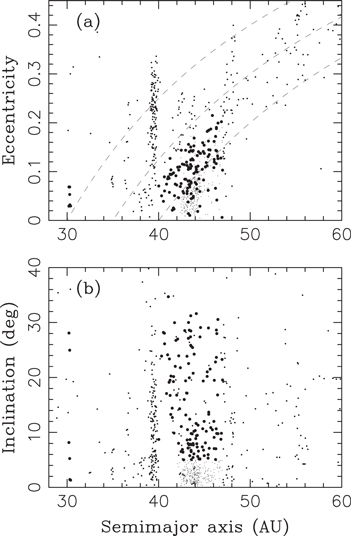
Figure 3. The same as Figure 1 but without labeling of different populations. This plot is useful for a visual comparison with the model results.
Download figure:
Standard image High-resolution imageWe used the CFEPS detection simulator (Kavelaars et al. 2009) to compare the orbital distributions obtained in our simulations with observations. CFEPS is one of the largest Kuiper Belt surveys with published characterization (currently 169 objects; Petit et al. 2011). The simulator was developed by the CFEPS team to aid the interpretation of their observations. Given intrinsic orbital and magnitude distributions, the CFEPS simulator returns a sample of objects that would have been detected by the survey, accounting for flux biases, pointing history, rate cuts, and object leakage (Kavelaars et al. 2009). In the present work, we input our model populations in the simulator to compute the detection statistics. We then compare the orbital distribution of the detected objects with the actual CFEPS detections using the Kolmogorov–Smirnov (K–S) test (Press et al. 1992).
This is done as follows. The CFEPS simulator takes as an input: (1) the orbital element distribution from our numerical model, and (2) an assumed absolute magnitude (H) distribution. As for (1), the input orbital distribution was produced by a short integration starting from the final model state of the Kuiper Belt. The orbital elements of each object were recorded at 100 year intervals during this integration until the total number of recorded data points reached ≃105. Each data point was then treated as an independent observational target. We rotated the reference system such that the orbital phase of Neptune in each time frame corresponded to its ecliptic coordinates at the epoch of CFEPS observations. This procedure guaranteed that the sky positions of the objects in Neptune’s resonances were correctly distributed relative to the pointing direction of the CFEPS frames.
The magnitude distribution was taken from Fraser et al. (2014). It was assumed to be described by a broken power law with  for
for  and
and  for
for  , where
  and
and  are the power-law slopes for objects brighter and fainter than the transition, or break magnitude
  , and H0 is a normalization constant. Fraser et al. (2014) found that
  ,
,  , and
, and  for the HCs. In the context of a model where the HCs formed at
  AU, and were implanted into the Kuiper Belt by size-independent processes (our integrations do not have any size-dependent component), the HC magnitude distribution should be shared by all populations that originated from
  AU (Morbidelli et al. 2009b; Fraser et al. 2014). We varied the parameters of the input magnitude distribution to understand the sensitivity of the results to various assumptions. We found that small variations of
  ,
,  , and
, and  within the uncertainties given in Fraser et al. (2014) have essentially no effect.
5. RESULTS
5.1. A Reference Case
We first discuss a reference simulation with slow migration of Neptune ( Myr,
Myr,  AU,
AU,  ,
,  ) to illustrate that the results of this model match the orbital structure of the Kuiper Belt, including the wide inclination distribution of the HCs and resonant populations. Later, in Section 5.3, we will explain how the results differ from the reference case when various model parameters, such as τ and
  , are varied.5
Figure 4 shows the orbital distribution of the model orbits obtained with
, are varied.5
Figure 4 shows the orbital distribution of the model orbits obtained with  AU and
  Myr. This figure can be compared to Figure 3, but note that some caution needs to be exercised in this comparison, because Figure 3 includes various observational biases, while Figure 4 does not. Also, the total number of points in the two plots is different (known KBOs with good orbits in Figure 3 and a fraction of the initial 106 disk particles in Figure 4).
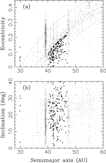
Figure 4. The orbital elements of bodies captured in the Kuiper Belt in a model with  AU and
  Myr. The HCs and NTs are denoted by larger symbols.
Download figure:
Standard image High-resolution imageThe model results in Figure 4 show a remarkable similarity to Figure 3. The orbital structure obtained in the model shows all main components of the Kuiper Belt, including the resonant populations, classical belt, scattered, and detached disks. The resonances such as the 5:4, 4:3, 5:3, 7:4, and 5:2 are also populated. The model orbits in the detached disk have perihelion distances reaching toward  AU, as they do in reality. Note that the CCs are not shown in Figure 4, because the model discussed here does not account for objects that formed beyond 30 AU (see discussion of the CCs in Section 1 and the description of the model in Section 3).
The model distribution of orbital inclinations in Figure 4 covers the whole interval between 0° and  . This is a notable result because the original disk orbits had
  . The orbital inclinations have therefore been significantly excited during the implantation process. The dynamical processes responsible for the implantation of objects in the Kuiper Belt and their effects on the orbital inclination are discussed in Section 5.2. Here we first more carefully compare the model distribution with observations. To do this, the model distribution shown in Figure 4 was passed through the CFEPS detection simulator. Figure 5 shows how the model detections compare with the actual CFEPS detections. The comparison is done separately for the 3:2 resonance and HCs. The reason for this is that the implantation process and stability properties can, and indeed do, produce differences between these populations. We do not show a similar comparison for other resonances, because the number of actual CFEPS detections in the 1:1, 2:1, and other resonances is very small (one to five objects detected) and a rigorous comparison is therefore not possible at this time.
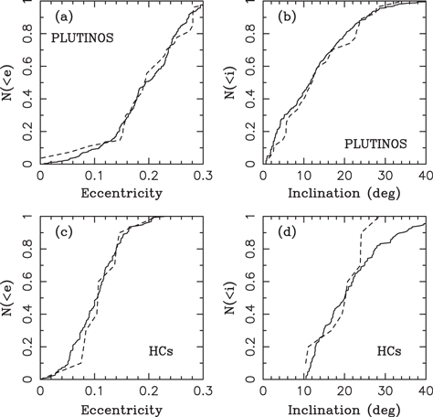
Figure 5. The cumulative distribution of eccentricities (left) and inclinations (right) for Plutinos (upper) and HCs (lower). The dashed lines show the actual CFEPS detections (29 Plutinos and 10 HCs with  ). The solid lines show the distributions of model bodies (
 AU and
  Myr) detected by the CFEPS simulator. Both the observed and model distributions plotted here therefore contain the CFEPS observational bias. For the HCs, we compare the distributions for
  to avoid any potential contamination of the detection statistics from the CCs, which are not modeled here.
Download figure:
Standard image High-resolution imageFigure 5 shows that the orbital distribution of the detected objects in the 3:2 resonance agrees with the distribution of the CFEPS detections. The K–S test indicates that the model and observed distributions shown in Figures 5(a) (eccentricity) and 5(b) (inclination) have 67% and 84% probabilities, respectively, of being derived from the same underlying distribution. This is very good agreement.6
The model distribution of inclinations obtained with  Myr is much wider than the one obtained for
  Myr (Figure 2), and matches observations very well. The eccentricity distributions are also very similar. Most Plutinos have
  (>80% of detections). This characteristic is a consequence of the implantation mechanism, where orbits are deposited into the 3:2 resonance from the scattered disk and retain large eccentricities (see Section 5.2). Note that, with
  AU, the 3:2 resonance is initially outside the outer boundary of the planetesimal disk. Plutinos are therefore not captured in our model from the low-eccentricity orbits as in, for example, Hahn & Malhotra (2005).
The agreement for the HCs is also good. The K–S test applied to the eccentricity and inclination distributions shown in Figures 5(c) and (d) gives 37% and 75% probabilities, respectively. As for the inclination distribution of the HCs, our model with  Myr and
  AU predicts that about 10% of the CFEPS detections should have
  , while no object was thus far detected by CFEPS with such a high inclination. This is not a problem, however, because the CFEPS detected only 10 HCs with
  , and the statistical constraints for
  are very weak. For
  , on the other hand, there are concerns with contamination from the CCs, which are not modeled here. The CCs should clearly have the dominant contribution to the statistics for
  . For
. For  , the situation is unclear. There are 11 CFEPS detections in this intermediate inclination range, which is similar to the number of detections for
  . In our model with
  Myr, however, these intermediate inclinations are not populated as much (we get about half of the expected detections). We believe this issue arises because our model with smooth migration of Neptune and a fixed value of τ is a somewhat inadequate approximation of the real evolution (see discussion in Section 6).
5.2. The Implantation Mechanism
We examined the orbital histories of test particles in the reference simulation and found that the implantation of bodies from  AU into the Kuiper Belt is in general a three-step process. The first two steps are common for the HCs and resonant populations; the third step is what distinguishes them. We first describe these steps and then illustrate them with a few examples. Specifically:
- the disk planetesimals are scattered by Neptune from <30 AU to >30 AU. Their distribution resembles that of the scattered disk in that they populate the region with
 AU and
  , where
  is the semimajor axis of migrating Neptune. Here we define the Intermediate Source Region or ISR as the orbital region with
  , where
  is Neptune’s aphelion distance, and
  AU. Most bodies implanted into the main belt evolved onto their present orbits via the ISR.
 - the scattered bodies evolve onto orbits with large libration amplitudes in mean motion resonances. The secular dynamics inside the mean motion resonances is complex, including large-amplitude Kozai, apsidal, and nodal cycles (e.g., Morbidelli et al. 1995; Nesvorný & Roig 2000, 2001). These effects can act to decrease the orbital eccentricity, thus decoupling the orbit from Neptune, on a characteristic timescale that is comparable to the period of the secular oscillations (>1 Myr).
- if Neptune were not migrating, the evolution described in Step 2 would be reversible and bodies would be released, sooner or later, back to the scattered disk. With Neptune’s migration, however, two additional alternatives can happen: (1) the orbit can evolve to a smaller libration amplitude and stabilize inside the resonance, or (2) it can be released from the resonance with low eccentricity and can end up on a stable, HC-like orbit with
 AU.
AU.
The three-step implantation mechanism described above was originally proposed in Gomes (2003) and Gomes et al. (2005). We will therefore call it the Gomes mechanism in the following. The Gomes mechanism was previously shown to work in several self-consistent simulations of the planetary instability/migration, where the disk particles carried actual mass (e.g., Gomes 2003). Because a relatively small number of disk particles was used, however, the statistics was not sufficient for a careful comparison with observations. Also, Neptune’s migration was unrealistically grainy in their simulations. Here we show that the Gomes mechanism works, with lower efficiency, even if Neptune’s migration is smooth.
Figure 6 shows an example of a disk particle that was captured on a high-inclination and low-eccentricity orbit in the main belt. This case is a clear illustration of the three-step Gomes mechanism described above. Initially, the particle starts with a = 28.5 AU, e = 0.04, and  . It is scattered by Neptune and evolves into the scattered disk, where it remains until roughly t = 13 Myr after the start of the simulation. During this first stage, the eccentricity and inclination are excited by encounters with Neptune. The orbit is then captured in the 2:1 resonance and remains in the resonance until t = 22 Myr (see the libration of the resonant argument in panel (f)). Once captured, it undergoes Kozai oscillations (see the libration of the perihelion argument in panel (e)). The eccentricity drops from 0.4 to 0.06 during this phase (13 to 22 Myr), while the inclination further increases from
  to
to  . Finally, about 22 Myr after the start of the simulation, the particle is released from the 2:1 resonance (see panels (b) and (f)) and lands on a main-belt orbit with a = 42.8 AU, e = 0.05 and
  . This orbit is stable for 4 Gyr.
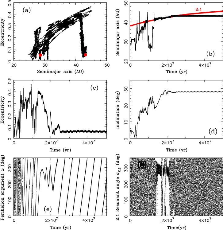
Figure 6. An illustration of the Gomes implantation mechanism. The panels show the (a) path of a disk particle in the (a, e) projection; the two red dots show the initial and final orbits, (b) semimajor axis, (c) eccentricity, (d) inclination, (e) perihelion argument ω, and (f) 2:1 resonant angle  , where λ and
  are the particle’s and Neptune’s mean longitudes, and ϖ is the particle’s perihelion longitude. After being scattered by Neptune and experiencing Kozai cycles inside the 2:1 mean motion resonance, the disk particle ends up on a high-inclination orbit in the main belt.
Download figure:
Standard image High-resolution imageFigure 7 shows an example of a disk particle that was captured on a high-inclination orbit in the 3:2 resonance. In this case, the scattering phase lasted until about t = 65 Myr. Both the eccentricity and inclination were strongly excited during this phase. At  Myr, the orbit entered into the 3:2 resonance. The resonant libration amplitude was initially variable but later evolved to become ≃100° (panel (f)). The 3:2 resonant orbits with such amplitudes are stable (Nesvorný & Roig 2000). Indeed, the orbit stayed in the 3:2 resonance for the whole duration of our integration (4 Gyr). During the capture into the 3:2 resonance the orbit started showing Kozai cycles (ω started librating in panel (e) while e and i in panels (c) and (d) exhibited signs of correlated oscillations). The Kozai oscillations with (full) amplitude of about 80° remained for the whole duration of the simulation. This case is reminiscent of Pluto, whose orbit also has Kozai cycles, but the final orbital inclination of this particle is considerably higher (
 versus Pluto’s
  ).
).
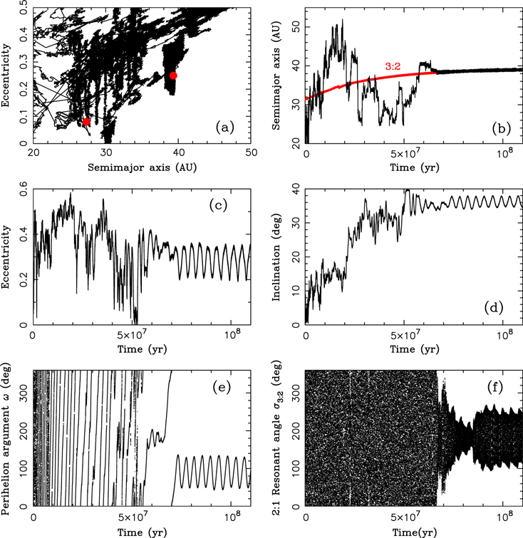
Figure 7. Capture of a disk particle on a stable, high-inclination orbit in the 3:2 resonance. The panels show the (a) path of the disk particle in the (a, e) projection; the two red dots show the initial and final orbits, (b) semimajor axis, (c) eccentricity, (d) inclination, (e) perihelion argument ω, and (f) 3:2 resonant angle  .
.
Download figure:
Standard image High-resolution imageFigure 8 is a case of Neptune Trojan. Akin to the example of the captured Plutino discussed above, the scattering phase lasts very long ( Myr). The eccentricity is excited but the inclination remains relatively low (<15°). Then, around t = 50 Myr, the orbit starts showing signs of the Kozai resonance (panel (e)) and undergoes two brief periods during which the 1:1 resonant angle librates (about t = 54 Myr and t = 60 Myr). The inclination rises and eccentricity drops in an anti-correlated pattern. The orbit is caught into the 1:1 resonance at
  Myr, eventually stabilizes with a very small libration amplitude (
 ) around the leading Lagrangian point L4, and remains there for 4 Gyr.
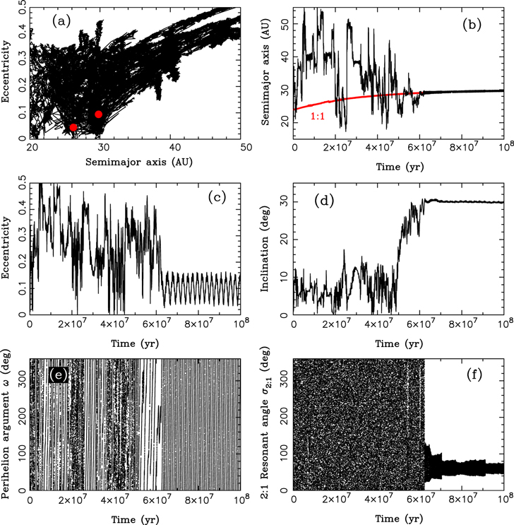
Figure 8. Capture of a disk particle on a high-inclination Neptune Trojan orbit. The panels show the (a) path of the disk particle in the (a, e) projection; the two red dots show the initial and final orbits, (b) semimajor axis, (c) eccentricity, (d) inclination, (e) perihelion argument ω, and (f) 1:1 resonant angle  .
.
Download figure:
Standard image High-resolution imageThe three examples discussed above were selected from hundreds of similar cases to illustrate the Gomes mechanism for capture in the main belt and resonances, and the high inclinations that these orbits can reach, if the migration of Neptune is slow and the scattering phase lasts for a long time. We found that the 2:1 resonance was typically involved in capture of orbits in the main belt, but resonances such as 7:4 or 9:5 also contributed. The orbits of the detached objects produced in our simulations follow a similar pattern, but the resonances responsible for raising their perihelia are different (e.g., 5:2, 7:3, 3:1). Moreover, relatively strong resonances such as the 3:1 are capable of producing the detached orbits with very large perihelion distances, and some of these orbits are reminiscent of that of 2004 XR190 (Buffy) (a = 57.7 AU, q = 51.5 AU; Allen et al. 2006; see Figure 4; also Gomes 2011).
5.3. The Inclination Distributions Obtained in Different Models
The results of our simulations show that the inclination distribution of bodies implanted in the Kuiper belt depends both on τ and  , but the main effect is that on τ. This is because the implantation of bodies in the Kuiper Belt happens on a timescale comparable to τ. With short τ, the implantation must be fast and Neptune does not have much time to raise the inclinations of the scattered bodies. Consequently, the inclination distribution of the implanted bodies is narrow and clustered toward
  . If, on the other hand, τ is long, the orbital inclinations of scattered objects can be substantially excited by Neptune encounters before these bodies are implanted into the Kuiper Belt. The inclination distribution of the implanted bodies is thus wide in this case. Figures 2 and 5 illustrated the dependence on τ for
  Myr and
  Myr. Figure 9 show this dependence for several additional cases.
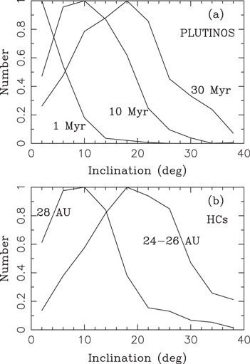
Figure 9. The dependence of the inclination distribution on τ and  : (a) Plutinos and (b) HCs. These distributions are the intrinsic distributions obtained in the model (i.e., they do not include any observational bias). The inclination distribution of Plutinos in panel (a) is sensitive to the assumed migration timescale. The labels in panel (a) denote the distributions obtained for different values of τ. In panel (b), we show the inclination distribution of HCs obtained with
  Myr. The two lines correspond to different starting positions of Neptune (
 –26 and 28 AU; the cases with
  and 26 AU were similar and were put together in this plot).
Download figure:
Standard image High-resolution imageThe inclination distribution of Plutinos obtained with different migration timescales is shown in Figure 9(a). The results obtained for  Myr and any
  are clearly a poor fit, because they indicate
  , while Plutinos have
  (Kavelaars et al. 2008; Gulbis et al. 2010; Gladman et al. 2012). The best-fit distribution for the case with
  Myr and
  AU is obtained for
  . When this case is compared to the CFEPS via the CFEPS detection simulator (Figure 10(b)), we find that it can be ruled out with 99.6% confidence. The results with
  Myr and
  AU can be ruled out at even higher confidence levels, because the inclination distributions of Plutinos obtained in those cases are narrower than the one obtained with
  Myr and
  AU. We conclude that fast migration timescales with
  Myr do not work for Plutinos.
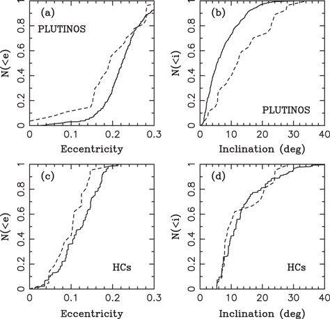
Figure 10. The cumulative distributions of eccentricities (left) and inclinations (right) for Plutinos (upper) and HCs (lower). The dashed lines show the actual CFEPS detections (29 Plutinos and 21 HCs with  ). The solid lines show the distributions of model bodies (
 AU and
  Myr) detected by the CFEPS simulator. Both the observed and model distributions plotted here therefore contain the observational bias of CFEPS. For the HCs we compare the distributions for
  to avoid contamination of the detection statistics from the CCs, which are not modeled here.
Download figure:
Standard image High-resolution imageLonger timescales produce better results. The case with  Myr and
  AU was discussed in Section 5.1 and clearly matches observations very well (Figure 5). Interestingly, the inclination distribution obtained in the model also depends on
  . For example, the inclination distributions obtained with
  Myr and
  AU or
AU or  AU are much narrower (
 ) than the one obtained with
  Myr and
  AU (
AU ( –20°). When compared to the CFEPS detections, these cases can be ruled out at a >99% confidence level. This happens because bodies tend to be captured relatively early in these simulations when Neptune’s migration rate is still substantial. In contrast, the long-range migration with
  AU offers more opportunity for capture at late times, and therefore leads to a wider inclination distribution that is more in line with observations. We therefore conclude from the inclination distribution of Plutinos that Neptune’s migration was slow (
 Myr) and long range (
 AU).
AU).
An additional argument that favors a long migration timescale comes from the eccentricity distribution of Plutinos. With  Myr, the model eccentricity distribution is skewed toward large values of e when compared to observations. This can be demonstrated by comparing the model to the CFEPS detections via the CFEPS detection simulator. For example, for
  Myr and
  AU (Figure 10(a)), the K–S test applied to the eccentricity distributions of the detected Plutinos gives only a 0.3% probability that the two distributions are the same. This mismatch is a consequence of step 2 of the capture process, discussed in Section 5.2, where there is not enough time available with rapid migration to decrease eccentricities. The eccentricities of captured objects therefore end up being too large.
We now move to discussing the HC inclination distribution. The HCs are deposited into the main belt ( AU) by mean motion resonances such as the 2:1 and 7:4. With
  AU, these resonances are located in the main belt with a = 44.4 AU and a = 40.7 AU, respectively. Therefore, in this case, the implantation of HCs into the main belt begins almost immediately after the start of a simulation (with a short delay required for Neptune to scatter bodies to the ISR; Section 5.2). The bodies implanted into the main belt during the initial stages will have small orbital inclinations and will skew the inclination distribution of HCs toward small values. Thus, even if long migration timescales are used in this case (e.g.,
  or 100 Myr), the inclination distributions obtained in the model end up being incorrect. See, for example, the case with
  AU and
  Myr in Figure 9(b). This specific case indicates
  –10°; it can be ruled out at a 99.8% confidence level from the CFEPS detections.
For  AU, on the other hand, the 2:1 and 7:4 resonances are at 38.1 and 34.9 AU. These resonances therefore cannot deposit bodies into the main belt during the initial stages of migration (because they are not located in the main belt during these initial stages). This means that the orbital inclinations in the ISR region can be excited by Neptune’s encounters before the main phase of the implantation starts. It starts when the 2:1 resonance moves beyond ≃40 AU, or equivalently, when Neptune moves beyond
  AU. When exactly this happens depends both on
  and τ. For example, with
  AU and
  Myr, Neptune moves past 25.2 AU at
  Myr after the start of migration. This delay is long enough to raise the mean orbital inclination in the ISR region to ≃10°. This explains why the orbital inclinations of HCs are generally higher when
  is smaller.
Figure 10 shows the eccentricity (panel (c)) and inclination (panel (d)) distributions of HCs obtained for  AU and
  Myr. While the eccentricity distribution is (slightly) discrepant when compared to the CFEPS detections, the inclination distribution looks good (K–S probability 29%). Unlike in Figure 5(d), panel (d) of Figure 10 compares the inclination distributions all the way down to 5°. The CFEPS inclination distribution is steep from 5° to 10°, and shallow above 10°. This may suggest that the underlying distribution is bimodal, perhaps because it resulted from capture at two different stages of Neptune’s migration (see discussion in Section 6). The model distribution obtained with
  AU and
  Myr is a good proxy for the overall shape of the CFEPS curve. We conclude from the inclination distribution of HCs that Neptune’s migration was slow (
 Myr) and long range (
 AU).
AU).
Figure 11(a) shows the mean orbital inclination of bodies in the ISR as a function of time. The mean inclination of the ISR population steadily increases with time. It is ≃5° at 106 years, ≃10° at 107 years, ≃15° at 3 × 10⁷ years, and ≃20° at 108 years. This makes it obvious that bodies captured in the main belt late will have, on average, larger orbital inclinations than bodies captured early, and explains the trends discussed above (see also Figure 12). Note, however, that the number of bodies available in the ISR drops for  Myr (Figure 11(b)). This is because bodies in the scattered disk evolve to very long orbital periods, or move to short orbital periods and are subsequently ejected from the solar system by Jupiter. This means that the number of bodies available for capture at very late times is relatively small. The very late captures (
 years) are therefore not very important for the overall statistics.
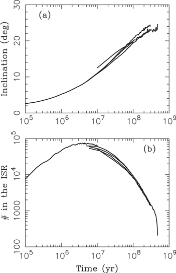
Figure 11. The mean orbital inclination and number of objects in the Intermediate Source Region (ISR), defined as  AU and
  . The lower panel shows that it takes 106–107 years to build up the ISR population, which then decays by about an order of magnitude over the next 108 years. The mean orbital inclination of the ISR population in panel (b) steadily increases with time. The different lines in panels (a) and (b) correspond to models with different τ and
  . The overall shape of the lines is insensitive to these parameters.
Download figure:
Standard image High-resolution image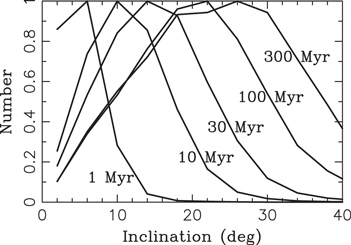
Figure 12. The inclination distribution of objects in the IRS for t = 1, 10, 30, 100, and 300 Myr after the start of Neptune’s migration. The plot shows how the orbital inclinations in the ISR increase as a result of encounters with Neptune. Here we used  AU and
  Myr.
Myr.
Download figure:
Standard image High-resolution imageIn summary, we find that the inclination distribution of the HCs is a reflection of the inclination distribution in the ISR, weighted by the number of bodies in the ISR, and time integrated over the capture window that depends both on  and τ. In addition, the inclination distribution becomes modified by the dynamical processes involved in step 2 of the capture process (see Section 5.2). Our main conclusion from the inclination constraint is that Neptune’s migration was long-range (
 AU), and that the migration timescale was long (
 Myr). The case with
  AU and
  Myr works relatively well for the HCs, but it fails for Plutinos (Figure 10). The case with
  AU and
  Myr works for HCs with
  deg and Plutinos. As we discuss in Section 6, the somewhat different timescales indicated by the HCs and Plutinos may be related to a two-stage migration of Neptune, with faster migration (
 Myr) during the first stage and slower migration (
 Myr) during the second.
5.4. The Implantation Efficiency
The efficiency of implantation of the disk bodies into the Kuiper Belt is a product of partial efficiencies of the three steps described in Section 5.2. During the first step, bodies from the disk at  AU are scattered by Neptune to
  AU, where they can be captured into resonances. The number of scattered bodies available for capture is a function of time (Figure 11(b)). The capture efficiency in a resonance mainly depends on the resonance strength (e.g., the strong 3:2 resonance is expected to capture more bodies) and Neptune’s migration speed. In step 2, the resonant bodies can evolve to orbits with lower eccentricities assuming there is enough time for the secular cycles to act. This depends on how Neptune’s migration timescale compares with the period of secular cycles in a specific resonance. Also, since the secular cycles depend on Neptune’s eccentricity, this stage is affected by Neptune’s eccentricity behavior during migration. Finally, whether a resonant orbit is or is not released from a resonance during step 3, is mainly influenced by Neptune’s migration speed (more bodies are released for higher speeds). Moreover, the implantation of bodies into the main belt occurs only when the relevant resonances are present in the
  AU region. For implantation via the 2:1 resonance, this requires that Neptune is beyond
  AU.
AU.
Some of the trends can be identified in our results. For example, with  AU, the efficiency of implantation on a stable orbit in the 3:2 resonance is
  for
for  Myr,
Myr,  for
for  Myr, and
  for
for  Myr. Also, for
  Myr,
Myr,  for
for  AU,
AU,  for
for  AU, and
  for
for  AU. Thus, a longer migration timescale leads to lower
  , and larger
  leads to higher
  . The trends for the implantation in the HC region are similar. For example, with
  Myr,
Myr,  for
for  AU,
AU,  for
for  AU, and
  for
for  AU.7
AU.7
In our preferred case ( AU and
  or 30 Myr), the main-belt capture efficiency is
  –4 × 10⁻⁴ for each initial particle in the original disk. With
 , the total mass of the hot population would therefore be
  –0.008
  . This is satisfactory when compared to
 estimated by Fraser et al. (2014), especially because Fraser’s estimate has a considerable uncertainty. Also, scaling from Jupiter Trojans, there should have been (3–
 planetesimals with absolute magnitude
  in the original disk (Nesvorný et al. 2013). With
  –4 × 10⁻⁴, our model would predict ∼7000–14,000 HCs with
  , while Adams et al. (2014) give 19,000 ± 5,000 from the Deep Ecliptic Survey (DES) for the whole population of the classical belt. This agreement is reasonable. (We note that the model estimates discussed here were obtained with
  and whenever
  stayed low during the migration. The cases with
  and/or the ones where the mean motion resonances between Uranus and Neptune acted to temporarily increase
  during the migration tend to produce larger
  , by a factor of a few, but more simulations would need to be done to establish this trend convincingly. The trend can be related to the dependence of the secular cycles inside the mean motion resonances on
  .)
.)
A major problem is identified when we consider the capture probability of the resonant objects. With  for the preferred case with
  AU and
  Myr, we would predict that the 3:2 resonance population should host ∼1.5–3 times more objects than the hot population in the main belt, while according to the CFEPS survey there are ∼3.5 times as many HCs as Plutinos (with absolute magnitude
  ; B. Gladman 2015, private communication). This would indicate
  (this estimate has a <50% formal uncertainty). The 3:2 resonance is thus obviously overpopulated in our simulations, roughly by a factor of 5–10. We call this the resonance overpopulation problem. This problem was already noted in many previous dynamical models of Kuiper Belt formation (e.g., Hahn & Malhotra 2005; Levison et al. 2008; Morbidelli et al. 2008).
There are several potential solutions to this problem. For example, we performed several simulations with  Myr and found that
  tends to be higher, and
  tends to be lower, than in the cases with
  Myr. For example, with
  AU and
  Myr (see Figure 13 for the orbital distribution of bodies obtained in this simulation), we found that
  and
and  , thus indicating
  . Also, with
  AU and
  Myr,
Myr,  and
and  , so
, so  . These ratios are more similar to the value
  inferred from observations. The case with
  AU produces a slightly wider inclination distribution than indicated by observations, while the one with
  AU produces a much narrower inclination distribution, thus suggesting the possibility that an intermediate value of
  26–27 AU would give the correct result. We do not give much emphasis to the cases with
  Myr in this paper, because it is not clear how these cases relate to our current models of the planetary instability and migration (e.g., they may require a very low mass of the planetesimal disk). New planetary instability simulations, with a focus on very slow migration timescales, will need to be performed. Another solution of the resonance overpopulation problem, which will also require additional modeling effort that goes beyond the scope of this paper, is discussed in Section 6.
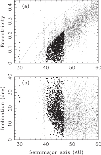
Figure 13. The orbital elements of bodies captured in the Kuiper Belt in a model with  AU and
  Myr. The HCs and NTs are denoted by larger symbols. Note that the number of bodies captured in the HC region is
  times larger than in Figure 4. The detached disk beyond 50 AU is also more populated and extends to
  AU. Both these results are a consequence of the very slow migration of Neptune assumed in this simulation.
Download figure:
Standard image High-resolution imageWe point out that the overpopulation problem is not specific to the 3:2 resonance. Instead, nearly all resonances are overpopulated. On the other hand, when we compare, relative to each other, the number of bodies captured in different resonances in our simulations, we find that these populations have roughly the right proportions. For example, for  AU and
  Myr, we find that
  and
and  . This is comparable to the resonance population statistics in the 3:2, 2:1 and 5:2 resonances discussed in Gladman et al. (2014) (even though the population in the 5:2 resonance was previously thought to be comparable to that in the 3:2 resonance; Gladman et al. 2012).
Another notable result obtained from our simulations concerns the NTs. Two problems were identified in previous modeling of the NT capture: (1) the capture efficiency obtained in the previous simulations was ∼2 orders of magnitude too high, and (2) the inclination distribution was too narrow (e.g., Nesvorný & Vokrouhlický 2009; Parker 2015). Related to (1), only five NTs were captured out of the original 106 disk particles for  AU and
  Myr. This indicates the capture probability
  and is more in line with observations (Alexandersen et al. 2014). As for (2), four of five stable NTs produced by the reference run have inclinations
  (Figure 4). This is encouraging, but better statistics will be needed to compare things more carefully.
6. DISCUSSION AND CONCLUSIONS
To summarize, here we investigated various models of Kuiper Belt formation by performing numerical integrations starting from an initial state with Neptune at  AU and a dynamically cold outer disk extending from beyond
  to 30 AU. Neptune’s orbit was migrated into the disk on an e-folding timescale
  Myr. By analyzing the inclination distribution of bodies implanted into the Kuiper Belt in different cases we found that the inclination constraint implies that
  Myr (slow migration) and
  AU (long-range migration). The models with
  Myr (fast migration) did not satisfy the inclination constraint, because there was not enough time for various dynamical processes to raise inclinations. The main assumption of this work is that the massive planetesimal disk (mass ∼20
  ) was truncated at
  AU, as constrained by the present orbit of Neptune (Gomes et al. 2004). If the massive disk continued beyond 30 AU, Neptune would migrate past 30 AU, and the distant disk would leave behind a large population of bodies on low-inclination orbits. This population would not look like the HCs, because of the problem with orbital inclinations, or the CCs, because the CCs only contain an estimated mass of
 (Fraser et al. 2014). The disk could have been truncated at 30AU by photoevaporation or a close stellar encounter (Adams 2010). The low mass continuation of the disk beyond 30 AU, a presumed source of the CC population, is considered in a companion paper (Nesvorný 2015).
The Gomes mechanism was identified here to have fundamental importance for the origin of dynamical structures in the Kuiper Belt. The basic requirement for the Gomes mechanism to work is that the migration timescale τ is comparable to, or longer than, the secular cycles inside the mean motion resonances such as 2:1, 3:2, 7:3, etc. With  AU, the 2:1 resonance is initially below 40 AU, sweeps over the main belt location at
  AU during Neptune’s migration, and is responsible for the delivery of most objects into the main belt. Since the secular cycles in the 2:1 resonance have a several-Myr period, τ needs to be at least several Myr for this to work. If, instead,
  Myr, objects can still be captured in the main belt region, assuming that Neptune had an orbit with substantial orbital eccentricity (Levison et al. 2008). In this case, orbits evolve from the scattered disk to the main belt by normal secular cycles outside the mean motion resonances (Dawson & Murray-Clay 2012). These cycles have a shorter period and work for shorter migration timescales.
A major problem with the high-eccentricity ( ) phase of Neptune is the opposing constraints from the hot and cold populations, as explained in Dawson & Murray-Clay (2012). Specifically, to preserve the CCs, the eccentricity of Neptune cannot be large and/or must be damped fast (Batygin et al. 2011; Wolff et al. 2012). To capture the HCs by the normal secular cycles outside the mean motion resonances, however, Neptune’s initial eccentricity must be relatively high at some point during Neptune’s migration. While these two constraints rule out most of parameter space, Dawson & Murray-Clay (2012), working under the assumption that the HCs were captured by the normal secular cycles, found solutions that satisfy both. This niche of parameter space is
  and
and  AU, essentially meaning that Neptune’s migration would have to be short range.
The beauty of the Gomes mechanism is that it works even if Neptune’s eccentricity was never large. This is because this mechanism does not rely on the normal secular eccentricity oscillations forced by eccentric Neptune on orbits outside the mean motion resonances. Instead, it appears as a product of large eccentricity oscillations due to the existence of large-amplitude secular cycles inside the mean motion resonances, akin to those first pointed out for the 3:1 Jupiter resonance in the asteroid main belt (Wisdom 1982). Here we showed that the Gomes mechanism is the dominant implantation mechanism from  AU in a regime where
  is low. Therefore, the argument of Dawson & Murray-Clay (2012) that
  is required to explain the HCs does not apply. On a related note, Levison et al. (2008) suggested that the existence of the detached disk with orbital perihelia extending to ≃40 AU is a consequence of an eccentric phase of Neptune, for Neptune to be capable of scattering objects to
  AU, and used
  in their simulations. Here we showed that the Gomes mechanism can produce the correct orbital architecture of the detached disk even if
  stays low, assuming that the migration timescale was long (e.g., Figures 4 and 13).
In this work, we stressed the importance of the inclination distribution of the KBOs. This is because the inclination distribution has been relatively well characterized from observations and can therefore be used to constrain models. We showed that the Gomes mechanism is capable of producing the observed wide inclination distribution from a dynamically cold disk at <30 AU, assuming that Neptune’s migration was long-range ( AU) and slow (
 Myr).8
The slow migration of Neptune is also consistent with other Kuiper belt constraints (e.g., Morbidelli et al. 2014) and with the present obliquity of Saturn (e.g., Boué et al. 2009; Vokrouhlický & Nesvorný 2015). Since the Gomes mechanism is insensitive to Neptune’s eccentricity, the eccentricity could have been negligible during Neptune’s migration in much the same way as originally proposed by Malhotra (1993, 1995) and later used by Hahn & Malhotra (1999, 2005) to model the origin of the Kuiper Belt from a disk at
Myr).8
The slow migration of Neptune is also consistent with other Kuiper belt constraints (e.g., Morbidelli et al. 2014) and with the present obliquity of Saturn (e.g., Boué et al. 2009; Vokrouhlický & Nesvorný 2015). Since the Gomes mechanism is insensitive to Neptune’s eccentricity, the eccentricity could have been negligible during Neptune’s migration in much the same way as originally proposed by Malhotra (1993, 1995) and later used by Hahn & Malhotra (1999, 2005) to model the origin of the Kuiper Belt from a disk at  AU.
AU.
How does this fit with the present ideas about planetary instability/migration occurring in the Nice model? The original Nice model, as proposed in 2005 (Tsiganis et al. 2005), was already shown to suffer from several fundamental limitations. For example, Jupiter’s migration cannot be smooth, because that would violate constraints from the terrestrial planets (Brasser et al. 2009, 2013; Agnor & Lin 2012), asteroid belt (Morbidelli et al. 2010), and the structure of secular modes in Jupiter’s orbit (Morbidelli et al. 2009a). A potentially more viable instability model, known as the jumping-Jupiter model, was later developed to avoid these problems (e.g., Brasser et al. 2009; Morbidelli et al. 2009a). In the jumping-Jupiter model, the four outer planets start in a compact resonant configuration at ≃5–12 AU and suffer a strong dynamical instability, during which Jupiter has encounters with Uranus and/on Neptune, and radially jumps. This turns out to resolve the problems of the original Nice model mentioned above. The main problem of the jumping-Jupiter model, as originally proposed, is that it is difficult to stabilize and circularize the orbits of Uranus and Neptune while matching other constraints as well (Nesvorný & Morbidelli 2012).
Levison et al. (2008) investigated the consequences of the strong instability model for the Kuiper Belt. They assumed that Neptune was scattered to  AU during the instability, where its initially eccentric orbit (
 ) was stabilized and circularized by a massive planetesimal disk. Subsequently, Neptune was assumed to migrate to 30 AU with
  Myr. The results of our work rule out this model. This is because, as we discussed above, the short-range migration of Neptune (
 AU) into a dynamically cold disk at
  AU would lead to a narrow distribution of orbital inclinations, in contradiction to observations. Moreover, to stabilize eccentric Neptune at
  AU, the disk would have to be massive (
 ; Nesvorný & Morbidelli 2012; hereafter NM12), and would produce fast migration of Neptune, thus leading to a double contradiction, because both τ and
  would be out of the plausible range identified here (Neptune’s migration needs to be slow, not fast, to explain the inclination distribution).
A new model of planetary instability has recently been proposed (Nesvorný 2011; Batygin et al. 2012; NM12). The model postulates that the early solar system had an extra ice giant, which was ejected into interstellar space during the instability. Figure 14 illustrates this possibility. In this model, five outer planets start in a relatively relaxed configuration with Neptune at  AU. The first thing that happens in the simulation is that Neptune migrates into the outer disk located at 24–30 AU. After Neptune reaches ≃28 AU, the instability happens, during which the extra ice giant has encounters with all the other outer planets, and is subsequently ejected by Jupiter. The main features of this model which are most relevant for the Kuiper Belt are (1) Neptune’s eccentricity and inclination are never large (
 and
and  ), (2) the initial mass of the outer disk at
  AU is relatively small (
 –20
–20  , NM12), therefore implying a slow migration of Neptune, (3) Neptune’s semimajor axis discontinuously changes (by ≃0.2–0.5 AU) when Neptune is at
  AU, as a result of one or two very close encounters with the ejected ice giant; the migration rate is slower after the jump than it was during the previous migration stage, and (4) the ejected ice giant briefly overlaps with the Kuiper Belt (Batygin et al. 2012).
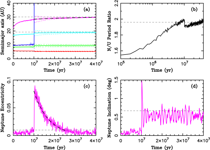


Figure 14. The orbital histories of the giant planets from the instability/migration model of NM12. In this example, the fifth giant planet was initially placed on an orbit between Saturn and Uranus and was given a mass equal to Neptune’s mass. The three inner planets were started in the (3:2, 4:3) resonant chain, and Uranus and Neptune on non-resonant orbits with  AU and
  AU. Ten thousand particles, representing the outer planetesimal disk, were distributed with semimajor axes
  AU, surface density
  , and low eccentricities and low inclinations. With the total disk mass
 , each disk particle has approximately one Pluto mass. (a) The semimajor axes (solid lines) and perihelion and aphelion distances (thin dashed lines) of each planet’s orbit. The inner ice giant was ejected into interstellar space at
  Myr after the start of the simulation. The final orbits of the four remaining planets are a good match to those in the present solar system (thin dashed lines). (b) The period ratio
  . The thin dashed line shows
  corresponding to the present orbits of Uranus and Neptune. Panels (c) and (d) show the eccentricity and inclination of Neptune’s orbit. The bold dashed lines in panels (a) and (c) approximate Neptune’s migration with
  Myr and damping of Neptune’s eccentricity with
  Myr. These long migration/damping timescales are characteristic for the migration/instability models from NM12.
Download figure:
Standard image High-resolution image

As for (4), we carefully looked into several instability cases from NM12 and found that the relevant period during which the ice giant’s orbit overlaps with the Kuiper Belt is too brief to significantly affect the orbits in the Kuiper Belt. Batygin et al. (2012), who found larger effects in about 50% of studied cases, did so probably because their work covered a broad range of possibilities, with some of their instability cases being somewhat too cataclysmic, in our opinion, to produce the solar system as we know it now. Items (1) and (2) present the right conditions for the Gomes mechanism to work and play a dominant role over other implantation mechanisms.
Unlike in the idealized case studied here, Neptune’s migration in Figure 14, and other cases reported in NM12, happens in two stages. During the first stage, that is, before the instability happens, Neptune migrates with  Myr for
 or
or  Myr for
 (these are the best exponential fits in the NM12 cases we looked at). During the second stage, that is, after the instability, Neptune migrates with
  Myr for
 or
or  Myr for
 . These best-fit τ values are only approximate, because the real migration is not exactly exponential, and the effective τ is typically longer as time progresses.
These timescales, and the long-range nature of Neptune’s migration in NM12, agree quite nicely with the constraints on Neptune’s migration derived from the Kuiper Belt in this work. This shows that the NM12 instability model, which was developed entirely from constraints unrelated to the Kuiper Belt, may have some relevance for the early evolution of the solar system.
The inclination distribution of the HCs may provide some evidence for the two stage migration of Neptune in the NM12 model. This is because the HCs can be captured into the main belt both during the first phase, when Neptune’s migration was faster, and during the second phase, when the migration was slower. The main implication of this is that the HCs can be a composite of two populations captured at two different stages. From the discussion in this paper, these populations are expected to have different inclination distributions, thus potentially explaining why the CFEPS detections of the HCs show different slopes for  (captures during the first stage) and
  (second stage). Also, Plutinos and other resonant populations, captured during the first stage, would be released when Neptune jumped during the NM12 instability. This could relieve the resonance overpopulation problem discussed in Section 5.4. The present resonant populations would then have to be captured entirely during the second phase, when the migration of Neptune was slower. This could explain why we are seeing a preference in our results for slightly longer τ values for Plutinos than for HCs (e.g., the case with
  Myr is works well for the HCs but does not really work for Plutinos; Figure 10).
Much work has yet to be done to fully understand the dynamics of the KBOs during Neptune’s migration, and how the history of Neptune’s orbit is constrained by the dynamical structure of the Kuiper Belt. Clearly, the idealized migration model studied here is a major simplification. We used it to highlight several interesting results that can be obtained within the framework of this model. We now plan to increase the realism of the model by considering the two-stage migration from NM12. We believe that this will be a crucial step toward resolving the resonance overpopulation problem that plagued previous studies of Kuiper Belt formation. In a companion paper, we study the implications of the NM12 instability model for the cold classical belt.
This work was supported by NASA’s Outer Planet Research (OPR) program. All CPU-intensive simulations in this work were performed on NASA’s Pleiades Supercomputer.9 We thank W. F. Bottke, L. Dones, B. Gladman, H. F. Levison, A. Morbidelli, D. Vokrouhlický, and an anonymous reviewer for helpful comments on this work.
Footnotes
- 1
- 2
Hahn & Malhotra (2005) started with 104 particles at
 AU, and a
  surface density profile. This means that they had
  particles in the inner disk between 20 and 30 AU. With the 10−3−10−4 capture probability, typical for the disk particles starting at 20–30 AU (see Section 5.4), the expected number of particles implanted in the Kuiper Belt from the inner disk in their simulations is 0.3–3. This shows that the statistics in Hahn & Malhotra (2005) was not good enough to investigate capture from the disk at 20–30 AU. Instead, their results were controlled by particles starting at
  AU. Hahn & Malhotra (2005) were aware of the previous work of Gomes (2003) and correctly pointed out the possibility that a more successful model can be constructed from a massive disk below 30 AU.
 - 3
- 4
The escape velocity from Pluto is 1.2 km s−1, about 20% of the Keplerian orbital speed at 25 AU. Therefore, eccentricities up to
 and inclinations up to ≃12° can be expected from a surface-grazing flyby near a Pluto-class object.
 - 5
These results are strictly reproducible. There is enough information given in Section 3 for anyone to repeat our simulations and confirm the results.
- 6
To be more precise, a K–S probability of 0.67 (or 0.84) means the following. Assume that there was a single parent distribution for both the model and the observations. In particular, the model was a random sample containing, say, J entries, while the observations contained K entries. If we were to generate two random representations of this parent population, one with J entries and one with K, there would be a 67% (or 84%) chance that the comparison between these random populations would be worse than what we have in Figure 5(a) (or Figure 5(b)). This holds despite the fact that these new distributions were directly derived from the parent. Therefore, the agreement between our model and the observations is very good. Indeed, any comparison with a K–S probability greater than ∼0.1 should be considered acceptable.
- 7
 (or
(or  ) is the probability that an original disk object ends up on a stable orbit in the 3:2 resonance (or in the HC region). We compute this probability by dividing the number of 3:2 resonant (or HC) bodies at the end of our simulations (4 Gyr) by the number of bodies in the original disk (106).
 - 8
Using an initially strongly excited disk is counterproductive, because this has the consequence, as shown by our additional simulations of Neptune migrating into a pre-heated disk, that the implantation efficiency in the main belt drops by a factor of several.
- 9