
Abstract
The previous presearch data conditioning algorithm, PDC-MAP, for the Kepler data processing pipeline performs very well for the majority of targets in the Kepler field of view. However, for an appreciable minority, PDC-MAP has its limitations. To further minimize the number of targets for which PDC-MAP fails to perform admirably, we have developed a new method, called multiscale MAP, or msMAP. Utilizing an overcomplete discrete wavelet transform, the new method divides each light curve into multiple channels, or bands. The light curves in each band are then corrected separately, thereby allowing for a better separation of characteristic signals and improved removal of the systematics.
1. INTRODUCTION TO KEPLER AND PDC
1.1. An Overview of the Kepler Data Pipeline
Kepler’s primary science objective is to determine the frequency of Earth-size planets transiting their Sun-like host stars in the habitable zone. This daunting task demands an instrument capable of measuring the light output from each of over 150,000 stars simultaneously, with an unprecedented photometric precision of 30 parts per million (ppm) at 6.5 hr intervals for 12th magnitude stars. The Kepler data pipeline is tasked with processing the Kepler data and detect the transiting planet signals.
The Kepler data pipeline is divided into several components in order to allow for efficient management and parallel processing of data (Jenkins et al. 2010a). Raw pixel data downlinked from the Kepler photometer are calibrated by the calibration module (CAL) to produce calibrated target and background pixels (Quintana et al. 2010) and their associated uncertainties (Clarke 2010). The calibrated pixels are then processed by the photometric analysis module (PA) to fit and remove cosmic rays and sky background and then extract simple aperture photometry from the background-corrected, calibrated target pixels5 (Twicken et al. 2010b).
The final step to produce light curves is performed in the presearch data conditioning module (PDC), where signatures in the light curves correlated with systematic error sources from the telescope and spacecraft, such as pointing drift, focus changes, and thermal transients are removed. Additionally, PDC identifies and removes sudden pixel sensitivity dropouts (SPSDs), which result in abrupt drops in pixel flux with short recovery periods up to a few hours, but usually not to the same flux level as before. These step discontinuities are identified separately from those due to operational activities, such as safe modes and pointing tweaks, and are mended using a sophisticated method (Kolodziejczak & Morris 2012). PDC also identifies residual isolated outliers and fills data gaps (such as during intraquarter downlinks) so that the data for each quarterly segment is contiguous when presented to later pipeline modules. In a final step, PDC adjusts the light curves to account for excess flux in the optimal apertures due to starfield crowding and the fraction of the target star flux in the aperture to make apparent transit depths uniform from quarter to quarter as the stars move from detector to detector with each roll maneuver. Output data products include raw and calibrated pixels, raw and systematic error-corrected flux time series, and centroids and associated uncertainties for each target star, which are archived to the data management center and made available to the public through the Mikulski Archive at STScI6 (McCauliff et al. 2010).
Data is then passed to the transiting planet search module (TPS) (Jenkins et al. 2010b) where a wavelet-based adaptive matched filter is applied to identify transit-like features with durations in the range of 1–16 hr. Light curves with transit-like features whose combined signal-to-noise ratio (S/N) exceeds 7.1σ for a specified trial period and epoch are designated as threshold crossing events (TCEs) and subjected to further scrutiny by the data validation module (DV). The 7.1σ threshold was set so that there is no more than one expected false alarm for Earth-like planets for the entire campaign assuming Gaussian statistics (Jenkins 2002). DV performs a suite of statistical tests to evaluate the confidence in the transit detection, to reject false positives by background eclipsing binaries, and to extract physical parameters of each system (along with associated uncertainties and covariance matrices) for each planet candidate (Wu et al. 2010; Tenenbaum et al. 2010). After the planetary signatures are fitted, DV removes them from the light curves and invokes TPS again, which searches over the residual time series for additional transiting planets. This process repeats until no further TCEs are identified.
1.2. Shortcomings of the Previous Version of PDC
Correction of systematic errors in Kepler light curves has seen a dramatic improvement with the new Bayesian maximum a posteriori (MAP) detrending algorithm in the completely rewritten presearch data conditioning (PDC) module of Kepler (Stumpe et al. 2012; Smith et al. 2012). Called PDC-MAP, it was first included in the 8.0 release of the Kepler Science Operations Center processing pipeline (Jenkins et al. 2010a) in September 2011. The main improvement of PDC-MAP over the previous PDC-LS (least-squares) method (Twicken et al. 2010a) is that the latter was prone to partially removing astrophysical signals and introducing significant noise for many processed light curves. The Bayesian MAP approach of the new algorithm makes it more robust against such overfitting. It can thus reliably remove the systematic errors, while at the same time preserving the astrophysical features of the light curves. Despite this and other significant improvements to PDC, the corrected time-series still exhibit some artifacts. First, about 20% of the light curves show some residual systematic errors. They also commonly exhibit incompletely corrected thermal transients from “Earth-point recoveries” (Stumpe et al. 2012) (see Fig. 1a). These are 100–200 cadence (2–4 days) long trends in the light curves that are caused by the thermal settling of the photometer after the monthly Earth-pointing events of the spacecraft, or after its quarterly roll (Haas et al. 2010). A similar type of artifact can be seen in the recovery from safe-mode events. For quarters that suffer from multiple interrupts of operation and commanded adjustments to photometer pointing, such as the highly challenging Kepler Quarter 2 (June 2009–September 2009), PDC-MAP will sometimes not perform error correction to a satisfactory degree (see Fig. 1b). Second, for roughly 5%–10% of targets the systematic error correction introduces high-frequency noise, which can make detection of planet transits or analysis of astrophysical signals more difficult. The introduced noise is generally small but can be quite large for a handful of targets.
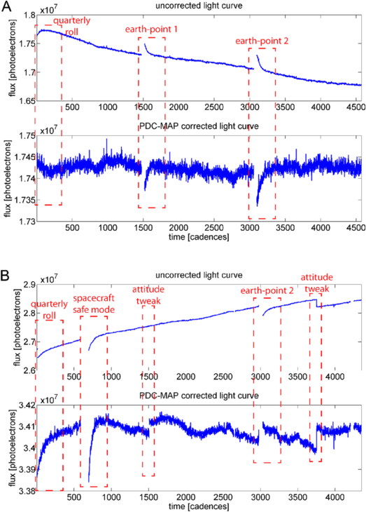
Fig. 1. Worst-case scenario examples of incomplete systematic error removal. (a) A common case where Earth-point recoveries, and to a lesser extent the quarterly roll recovery, are not completely corrected. (b) A light curve from Quarter 2, with multiple imperfect corrections of safe modes, Earth-points, quarterly rolls, attitude tweaks and loss of fine point.
The above artifacts have the same origin: the MAP cotrending basis vectors, which are used to fit and remove the systematic errors in the light curves, usually contain features on very different time scales (see Fig. 2)—ranging from only a few cadences or hours (e.g., Argabrightenings (Witteborn et al. 2011)), over several days (e.g., Earth-point recoveries or reaction-wheel zero crossings [Stumpe et al. 2012]), to several weeks or even months (e.g., long trends due to differential velocity aberration and focus changes). Thus, corrections of errors on different scales cannot be independent, and so the removal of errors on one scale can have the side-effect of injection or incomplete removal of errors on another scale. As a second issue, some basis vectors contain very high-frequency components and noise. This leads to injection of high-frequency noise in the MAP correction. In mathematical terms, these issues can be regarded as a consequence of the set of cotrending basis vectors not forming an independent basis. The basis set is quite complete, in the sense that all the trends are represented in the basis vector set. Because they are convolved with each other, however, proper removal is not always possible. Simply increasing the number of cotrending basis vectors in the fit does not only quickly render it computationally infeasible, it has further not been found to significantly increase the overall performance of the systematic error removal (see § 3.4). If anything, increasing the number of basis vectors just results in more stellar features being removed.
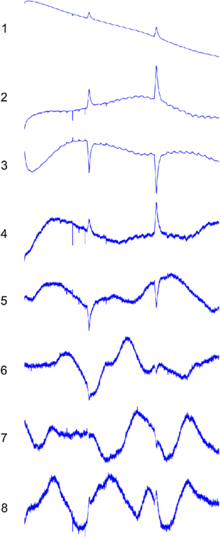
Fig. 2. Example of a set of eight non-multi-scale MAP cotrending basis vectors (shown here for module output 7.3, Quarter 10) exhibiting the issues motivating the development of multiscale MAP: systematics are present in the same basis vector on a different time scale, and also the presence of high-frequency noise for the latter basis vectors.
We note that, since the Earth-point recoveries are the most obvious type of residual systematic errors in PDC-MAP, other approaches to mitigate their detrimental effect on the light-curve quality are conceivable. One approach would be to simply ignore the recovery phase and discard the respective cadences (Petigura & Marcy 2012). However, this would discard a substantial portion (about 10%) of all data points in each time series. It is important to realize that this loss could not be mitigated by longer Kepler observation times, because the recurring gap in the data would create a blind spot for planet transits that have a matching epoch and period to fit into these gaps. This point is further exacerbated now that primary mission fine-point data collection has ended for the Kepler spacecraft.7 Another conceivable approach could be to change the unit of work in Kepler PDC from quarter-long light curves to only month-long light curves. This would yield only one strong thermal transient signal at the beginning of the time-series, which might be easier to correct. However, this approach would limit the maximum length of systematic errors PDC can identify and correct to one month, because the maximum length scales of stellar features that can be preserved are limited by the length of the unit of work. Further, this approach would only work for recoveries from scheduled events (such as the monthly Earth-point), but not with recoveries from unplanned events such as safe-modes or loss of fine-point (see Quarter 2, for instance), which lead to similar recovery artifacts. To avoid these and other potential shortcomings of simpler approaches, we have designed a more sophisticated algorithm which sacrifices neither data quality nor quantity.
2. The Solution: Multiscale Error Correction
In this work we present a solution to these problems, which we have first implemented as a major improvement to Kepler PDC in version 8.2. The approach we take is to perform a separation of scales in the time-series, such that small-scale features and large-scale features are described by different cotrending basis vectors. Figure 3 illustrates this approach: each time-series is split into multiple channels (bands). The set of light curves in each band is corrected separately with the MAP error correction algorithm (Smith et al. 2012). The corrected light curve bands are then combined again to generate the corrected light curves. Since many different systematics occur on different time scales this “band-splitting” is useful in isolating the systematics. For example, thermal stresses on the spacecraft due to its orbit about the sun results in systematics on a yearly time scale, whereas the reaction wheel heater cycling occurs on a 3 day cycle. These two systematic affects are independent of each other, but since they occur on different time scales they can be isolated using the band-splitting method described below.
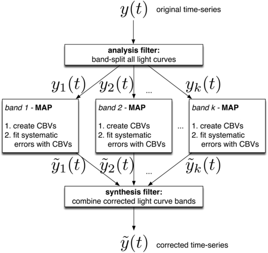
Fig. 3. Multiscale PDC-MAP correction scheme. Each light curve y(t) is decomposed into k bands yi(t) (i = 1…k) using an analysis filter. The MAP systematic error correction algorithm is performed on each band yi(t) separately to generate the corrected light curve band  . Finally, the corrected light curve bands are combined again with a synthesis filter, yielding the corrected light curve
  .
.
To decompose each light curve into a set of light curves on dyadic (power of two) scales, we use an overcomplete discrete wavelet transform (Percival & Walden 2000). As a joint time-frequency representation, it is a natural choice for such a multiscale analysis. Similar to the short-time Fourier transform (STFT), the wavelet transform is a windowed analysis technique that allows for the analysis of nonstationary signals. In contrast to the STFT, however, the wavelet transform uses variable-sized windows to tile the time-frequency plane. In particular, the wavelet transform employs basis functions Ψτ,λ(t), which are scaled (by λ) and shifted (by τ) versions of a mother-wavelet Ψ(t), and which are finite and vary in both duration and bandwidth. Because of these properties, the frequency and temporal resolution vary across scales, in such a way that their product (the area of the time-frequency tile) is constant at all scales. This property, that the bandwidth at each channel divided by its center frequency is constant, is also known as the “constant quality” (constant-Q) property (Vetterli & Kovacevic 1995). As a result, the wavelet decomposition achieves the best time resolution at the shortest scales (highest frequencies) and the best frequency resolution at the longest scales (lowest frequencies).
Convolution of a signal y(t) with the wavelet basis functions Ψτ,λ(t) via the “wavelet transform”, WT, produces a series of wavelet-coefficients w(τ,λ) for each wavelet basis function (characterized by its shift τ and scale λ),

The scales are chosen as powers of two (λi = 0,1,2,4,8,…,N), leading to a doubling of the characteristic scale in each band and the constant-Q property. By taking all possible shifts in each band (τj = 1…T, where T is the length of the discrete input time series y(t)), we perform an overcomplete discrete wavelet transform (Percival & Walden 2000). Figure 4 shows the original light curve and the set of wavelet coefficients for the light-curve. The wavelet coefficients w(τ,λ) are proportional to the power of the signal at each particular shift τ and scale λ. Here we can see distinct events, such as that the Earth point thermal recoveries are spread out as we move to longer length scales. Long-term trends are in the longest scale (1024 cadences) however the colormap has been saturated at large values in order to show the details at smaller scales. Intermediate length features in the 128, 256, and 512 cadence scales. High-frequency features are in the 1–4 cadence scales. Also note the single spike in the light curve at cadence 1150 exhibits itself as a streak along many scales.
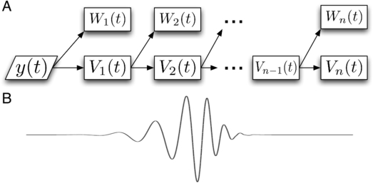
Fig. 4. Wavelet analysis of the light curve for Kepler ID 5356467 Quarter 10. Top: Input light curve flux. Bottom: Wavelet coefficients w(τ,λ), where the shift τ is plotted horizontally and the scale (2λ-1) is on the vertical axis. Distinct features in the light curve can clearly be seen extending across multiple scales in the wavelet coefficients. To show details at shorter scales the 1024 scale is saturated in the colormap.
The wavelet coefficients themselves are not used for MAP directly, but instead we immediately perform a reverse wavelet transform in each band, thereby reconstructing the light curve in the time-domain, albeit band-split. It is this band-split signal in the time domain to which MAP is applied. With the overcomplete wavelet transform, the reconstruction of the whole signal y(t) from the wavelet coefficients w(τ,λ) can be done by applying the reverse transform WT-1 in each band i separately,

Taking the linear sum over yi(t) for all scales i would result in the original light curve before band splitting,

However, because this reconstruction as well as the MAP correction are both linear operations, we can perform a MAP correction (Smith et al. 2012) in each band separately,

and then take the sum of the corrected light curve bands  to obtain the total corrected light curve
  :
:

Note that even though the MAP operation is linear it is not commutative,

and so the band-split msMAP operation results in a distinct correction to regular MAP.
The process of a wavelet transformation followed by a reverse wavelet transformation can be interpreted as an octave filterbank that iteratively splits a signal Vi(t), with the input signal y(t) = V0(t), into a “detail” layer Wi+1(t) and an “average layer” Vi+1(t), as illustrated in Figure 5a. The ith “detail” layer captures changes in the input signal on a scale of 2i-1, while the ith “average” layer captures smoothed structure on a scale of 2i. The perfect reconstruction property of the wavelet decomposition guarantees that the original signal is the sum of the “detail” layers and the last “average” layer:
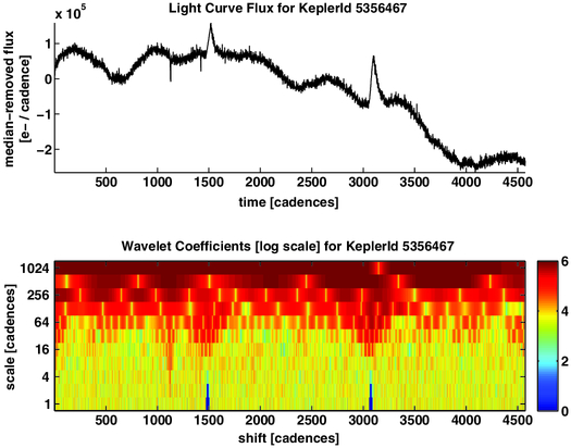
Fig. 5. Illustration of the wavelet transformation represented as (a) an octave filterbank which decomposes the input signal into successive “detail” layers Wi(t) and “average” layers Vi(t), and (b) as a Daubechies wavelet, which is chosen as the mother wavelet in this work.

In light of equation (7), we can now refer back to Figure 4 to discover that the plotted wavelet coefficient scales 1–512 are the “detail” layers Wi(t), whereas the 1024 scale is actually the final “average” layer Vn(t).
As the mother-wavelet, we use the Daubechies 12-tap wavelet (Feauveau et al. 1992) (see Fig. 5b). It is important to note that the MAP fit is not performed in the wavelet-domain, but in the regular time-domain. The process is illustrated in Figure 6. A further detail not shown in the figure is that the uncertainties are split using the same method as the light curve data and then the propagation of uncertainties method as used in MAP (Smith et al. 2012) is applied in each band. The uncertainties are then combined to produce the output uncertainties for msMAP.
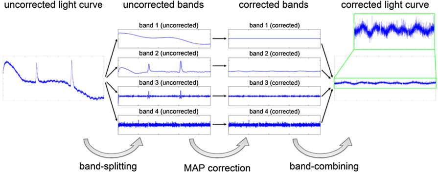
Fig. 6. Bandsplitting example.
A wavelet decomposition of a typical light curve into its channels (1–11) is shown in Figure 7. Each channel has a characteristic scale that is twice as large as that of the next channel. Rather than performing a MAP correction directly on each individual channel, however, it is preferable to group a number of adjacent channels together and perform the MAP correction on each of these combined bands. In the case illustrated in Figure 7, for instance, 11 channels are combined into four bands. Aside from the MAP correction being relatively expensive to perform on 11 channels individually (Stumpe et al. 2012), we found that the correction performance is better when grouping channels together this way. The main reason for this is that when having many bands, the errors and features in the time-series get spread across band boundaries and are distributed across multiple bands. Thus, different parts of the same feature are subjected to different MAP fits, which can lead to imperfect corrections. We therefore choose the groupings so that characteristic features are wholly contained in a single band. Also, overfitting can occur if all 11 channels are fit separately due to the large number of degrees of freedom in the correction (see § 3.4).
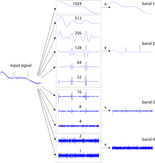
Fig. 7. Decomposition of the input light curve (left) into a set of subbands with dyadic scale. Multiple subbands are combined (dashed boxes) by summation to yield the final bands (right). The numbers on the subbands denote the characteristic scale in units of cadences for the respective subband.
Figure 8 gives the first four MAP cotrending basis vectors in a three-band decomposition. The cotrending basis vectors in the different bands separate the scales of the systematic errors very nicely, allowing independent correction of the errors. In particular, band 1 contains long-term trends, band 2 contains artifacts of medium duration (such as the Earth-point recoveries and the 3-day reaction wheel cycle), and band 3 contains very high frequency features such as Argabrightenings. For band 3, which contains the characteristic scales of 1 and 2 cadences, MAP finds no significant systematic signals among the light curves (using an S/N test), and therefore vetoes all cotrending basis vectors. With no surviving cotrending basis vectors, no correction is performed in the shortest band, and the light curve signals are simply preserved from this shortest band. Consequently, the noise is separated from the systematic errors and thus there is no injection of high-frequency noise as a side-effect to removing the systematic errors. Some subtle features are apparent in band 3, and future improvements to msMAP involve extracting these systematic signals (see § 6).
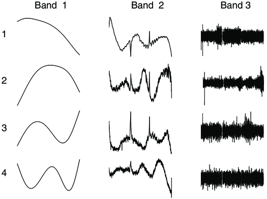
Fig. 8. The first four MAP cotrending basis vectors in a three-band decomposition for Quarter 5 Module Output 7.3. Signals are principally in the first two bands, but there are slight signals in band 3, which are however barely above the noise floor.
3. Choice Of Parameters
The PDC-MAP algorithm has a set of parameters, such as the number of basis vectors and certain weighting coefficients, which can be chosen by the pipeline operator to achieve optimal correction performance (Smith et al. 2012). The multiscale extension presented here introduces more parameters and detail choices for the algorithm, which have to be characterized and optimized for correction performance. In particular, the most important parameter choice is the grouping of channels to combine into bands, which determines the number of bands as well as the scale range of each band. Moreover, the PDC-MAP parameters can be chosen independently for each band, leading to a significantly larger parameter space. We have tested a wide range of parameter choices to investigate their effects on the correction performance, and discuss our main findings here.8
3.1. Number of Bands
The number of bands directly determines the number of degrees of freedom for the overall MAP correction, and thus the “flexibility” of the fit. The two border cases are (1) performing a MAP fit on each channel without any grouping of bands, and (2) grouping all channels together into one band. The latter is equivalent to the regular version of PDC-MAP. We found that the best results are usually achieved by using a decomposition into either three or four bands. Fewer bands lead to residual artifacts as in the case of regular PDC-MAP, whereas more than five bands can lead to unconstrained fits, splitting of features across multiple bands, and either overfitting or introduction of artifacts in extreme cases. A general trend we observed is that time series which suffer from more and stronger artifacts (e.g., heavily corrupted observation quarters such as Quarter 2, or more sensitive CCD channels) benefit from corrections with four or even five bands, whereas for time series with fewer systematic errors, three bands are usually the best choice. To perform a comprehensive comparison between three-band versus four-band decomposition, we performed both on all CCD channels of quarters Q5–Q8, (i.e., a time span of one full year to exclude potential seasonal effects), and evaluated the correction quality using visual investigation of a subset of light curves, as well as with the PDC goodness metric (including a new Earth-point goodness component; see § 4.2) to obtain aggregate statistics.
The PDC goodness metric (Stumpe et al. 2012) quantifies the performance of the cotrending in PDC with four basic performance qualities: (1) removal of target-to-target correlations, (2) injection of noise, (3) preservation of stellar signals, and (4) removal of Earth-point thermal recoveries. The study concluded that the absolute magnitude of the differences in the goodness metric between the three-band and four-band decomposition is only marginal and is almost negligible in practice. This is evident when comparing the total goodness between three and four bands, as shown in Figure 9. This shows that for almost all CCD channels, the difference between three-band and four-band average correction performance is on the order of only 1%. In the visual comparison of the corrections for individual targets, we did find some examples where the correction was better using four bands (see Fig. 10a for an example), and in rare cases the four-band correction was significantly worse than the three-band correction (see Fig. 10b for an example). The bottom line of this comparison is that either three or four bands should be used, and they both yield very similar correction performance.
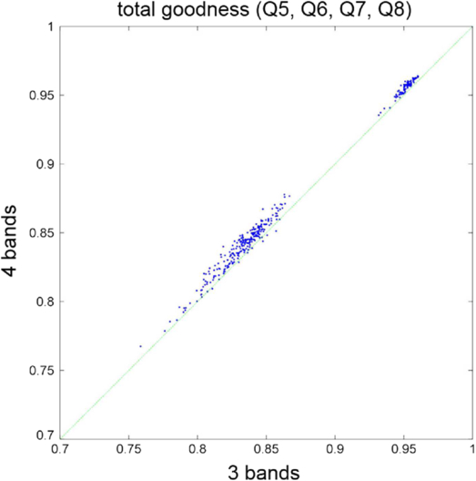
Fig. 9. Comparison of the total goodness between a three-band vs. a four-band correction for all four quarters Q5–Q8.
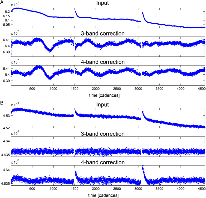
Fig. 10. Comparison of a three-band vs. a four-band correction. (a) A four-band correction can sometimes lead to better results when the three-band correction has residual systematic errors. (b) On the other hand, four-band corrections can sometimes introduce artifacts. Both of these cases are rare, and usually both corrections perform similarly well.
3.2. Channel Grouping, Band Boundaries
The second central parameter choice is which channels and thus characteristic scales to group together and treat in the same MAP fit. For example, Figure 7 shows a decomposition where band 1 contains only the scale of 1024 cadences, band 2 contains the scales 512, 256, 128, 64, 32, band 3 contains the scales 16, 8, 4, and band 4 contains the scales 2, 1. We abbreviate this here as “(1024/512,256,128,64,32/16,8,4/2,1)”. Alternative four-band decompositions could be (1024/512,256,128/64,32,16,8,4/2,1) or (1024,512,256/128,64,32/16,8/4,2,1). In the course of this parameters study, we systematically varied the band boundaries for three-band and four-band decompositions, and identified two important factors.
First, the most important separation is between very long trends on the scale of weeks or a months (>800 cadences), and the 3-day (≈150 cadences) Earth-point recoveries, as well as reaction wheel desaturation cycles (Stumpe et al. 2012). It is therefore favorable to not have the 1024 channel in the same band as the 256 or 128 channel. Second, it is beneficial to have a separate band for very short scale features, such as the (2,1) band. This helps to decouple the noise from the correction of midscale or large-scale errors and helps to reduce the problem of noise injection in PDC-MAP significantly. In fact, since MAP automatically chooses the optimum number of basis vectors (Smith et al. 2012), and in multiscale MAP this is done in each band separately, the number of basis vectors for the shortest (2,1 cadences) band is always found to be zero, and so no cotrending is performed on this scale at all. The light curves are consequently unchanged for the shortest band preserving all short (1–2 cadence) signals in the light curves. To a lesser extent, we also found that having most of the spectrum of a particular systematic error in the same band helps to improve the correction quality. For instance, as seen in Figure 4, Earth-point recoveries have a strong signal on the scales (128,64,32). Since Earth-point recoveries are the most prominent residual systematic errors in PDC-MAP, grouping the channels with scales (128,64,32), and possibly also 256, in the same band appears useful for the correction. Based on these observations, we found (1024/512,256,128,64,32/16,8,4/2,1) to be a good four-band decomposition and (1024/512,256,128,64,32,16,8,4/2,1) to be a good three-band decomposition for most cases. However, as with the number of bands, the overall correction performance was not overly sensitive to this parameter choice within small variations.
3.3. Modification of MAP Parameters
An investigation of several MAP parameters, in particular the number of basis vectors per band, showed that most MAP parameters should remain unchanged and the same for each band. One parameter which had to be changed is the light-curve normalization method for the singular value decomposition and for the MAP fit (see Smith et al. [2012] for details). We use normalization by the mean only in the longest-scale band, because the other bands have zero mean. Instead, the medium-scale bands are normalized by the standard deviation of each light curve. With no long-term trends (or high-frequency noise) in the medium-scale bands, the standard deviation remains the best metric for normalization. The shortest scale band is normalized by the noise floor, which is estimated by the first differences between the cadence flux values. Another MAP parameter that must be tuned is the prior PDF goodness weighting component in the prior weighting calculation (see again Smith et al. [2012]). The gain in the prior PDF Goodness must be increased for the shorter bands relative to the stellar variability component of the prior weight.
A final noteworthy parameter change is that we perform a robust least-squares fit, rather than a full MAP-fit, in the longest-scale band. We found that a MAP fit in the longest-scale band can lead to artifacts in the form of low-frequency waves. These waves, which are usually only very small, are exacerbated by nonideal MAP fit priors in this band. In the case of bad priors, MAP usually sets the weight of the prior to zero, effectively reverting back to a robust least-squares fit (Smith et al. 2012). This successfully eliminates the artifact. However, in the case of the longest scale band, even a slight error on the prior can “pull” the posterior fit too far away from the conditional, resulting in an artifact residual wave in the light curve. The robust least-squares fit does introduce the risk of overfitting but we have found that the additional attenuation of long period signals in msMAP is small compared to regular MAP and acceptable given the much greater performance at shorter frequencies relevant to transit detection.9 Therefore, the default configuration is to perform a robust least-squares fit in the longest band. It is difficult to distinguish between systematic and intrinsic stellar signals at periods approaching one observing quarter in length, and so we believe the forced robust fit is acceptable, but we are investigating methods to improve the prior in the longest-scale band and preserve signals out to longer periods.
3.4. Discussion of Alternative Approaches
In addition to the optimization of parameters, we have also investigated alternative approaches and modifications to the algorithm. We will briefly describe the most relevant ones here.
3.4.1. Increasing the Number of Basis Vectors without Employing a Multiscale Framework
As the systematic errors we want to correct are on a variety of different time scales, a multiscale approach seems very natural. However, it is an interesting question whether the dramatic performance improvements achieved by our new algorithm are really due to the multiscale aspect of our approach. One side effect of the multiscale approach is that it effectively increases the total number of basis vectors, and thus the degrees of freedom in the MAP fit. Could similar performance be achieved by simply increasing the number of basis vectors in a regular MAP fit? We have tested the effect of the number of basis vectors in the original PDC-MAP work and found that going beyond eight basis vectors does usually not improve the correction performance. PDC-MAP chooses the optimal number of basis vectors automatically based on the eigenvalue spectrum (Smith et al. 2012), and tests where we explicitly forced the number of basis vectors to be larger (e.g., 16 or 24) did in fact not show any performance improvement.
3.4.2. Using Multiscale Basis Vectors in a Joint Fit
Another conceivable option, and in fact an alternative design that we tried in the beginning, would be to generate the basis vectors separately for each band—as is done here—but instead of performing one MAP fit in each band separately, just do one MAP-fit with the joint set of basis vectors on the original unsplit light curves. We have tried this approach, but found that it does not perform well. Almost all light curves showed strong residual systematic errors or even injection of artifacts, such as enhancement of the Earth-point thermal transients. This is due to overfitting, since the number of basis vectors used is expanded by a factor of three. Thus, the basis vectors for each band should be fit separately on band-split light curves. Essentially, this approach suffers from similar problems as the original PDC-LS (Twicken et al. 2010a), the predecessor of PDC-MAP, and these deficiencies were the initial motivation to develop the latter.
3.4.3. Processing of All Channels without Grouping Them into Bands
One central step in our algorithm is the grouping of several adjacent octave channels into bands (see Fig. 7). This additional step introduces additional parameters (i.e., the band composition; see § 3.2) and it is questionable whether a simpler design without this step would work equally well. We tested this and performed a msMAP correction on all individual channels, but found that the results are significantly worse. In particular, using such a large number of bands renders each individual fit too unconstrained and leads to substantial overfitting and removal of many astrophysical signals. In some rare cases where Earth-point artifacts were not fully corrected with a three-band or four-band fit, this approach performed better at removing those artifacts, but at the expense of severe overfitting.
3.4.4. Choice of the Wavelet Family for Band-splitting, and Alternative Filterbanks
Daubechies-wavelets have several useful characteristics that make them a common choice for a mother wavelet. One of their major advantages is that an orthogonal set of Daubechies-wavelets can be created (Feauveau et al. 1992), which renders the synthesis process into a simple summation of the individual bands—a fact that we exploit here (eqs. [3] and [5]). Two other commonly used wavelet families are the simple Haar-wavelets and the Gabor-wavelets. Both are widely used in image processing and computer vision, for instance for feature-based object detection (Zeng et al. 2009). Gabor-wavelets have the disadvantage that they are not orthonormal, and thus the signal synthesis is a more complex operation. While this does not play a role in its intended application, where synthesis is usually not required, it would complicate processing in our case application here. Therefore, we have only investigated using Haar-wavelets as alternative to Daubechies-wavelets. The correction performance using Haar-wavelets was similar but inferior in most cases, most likely due to it having poor frequency response, which results in large leakage out of each band. Finally, simpler approaches for constructing the filterbank for band-splitting are also conceivable. In particular, we tested band-splitting using mean-filters, median-filters, Gaussian-filters, and Savitzky–Golay filters (Savitzky & Golay 1964), but we found that the overall correction performance was best when using wavelets. This result is not surprising, given that the scale-invariance of wavelets makes them intrinsically suited for any multiscale-related problems and accounts for their great success in these applications.
4. Further Algorithm Details
4.1. Cases of Bad Corrections: Vetting
In some cases (1–2% of all targets) it can happen that msMAP fails in correcting a light curve, and that systematic errors or noise are enhanced. Fortunately, these bad corrections are usually not subtle imperfections, but rather epic failures that are obvious upon inspection. In these cases, the more conservative correction of the original PDC-MAP usually yields a better correction. Figure 11 shows two representative examples of such cases. In the first case (Fig. 11a), the msMAP correction (lower panel) substantially enhances the Earth-point recovery artifacts and the 3-day reaction wheel cycle. In contrast, the regular PDC-MAP correction (middle panel) does not correct the Earth-points recoveries completely, but the overall correction quality is much better. In the second case (Fig. 11b), the msMAP correction shows significant injection of high-frequency noise, and also exhibits overfitting. The regular PDC-MAP correction, in contrast, appears near flawless. The main cause for these bad corrections are bad priors for the MAP fit (Smith et al. 2012), mostly in the middle bands. Many of the targets with bad corrections are very bright (magnitude 10 and lower). Since the magnitude has a strong influence on the MAP prior, the sparsity of correlated targets at low magnitude, which are used to generate the prior, can explain the bad priors for many of these these targets.
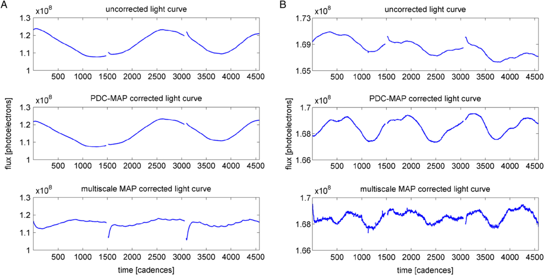
Fig. 11. Two cases of bad corrections with msMAP, showing strong residual artifacts such as Earth-point recoveries and 3-day reaction wheel cycles (a), as well as noise-injection and overfitting (b).
Our new version of PDC tries to identify these bad corrections using the goodness metric (Smith et al. 2012), and in the case of a bad correction reverts back to a regular PDC-MAP correction. For this purpose, a regular MAP correction is performed for each target in addition to the msMAP correction. Then the goodness metric is calculated for both corrections, and PDC decides for each target individually whether it should use the msMAP correction or revert to regular MAP. The process is illustrated in Figure 12. Decisions for each target are made on a quarterly basis, one quarter being one unit of work for PDC, and so a multiquarter stitched light curve can have PDC data for individual quarters using both regular MAP and msMAP processed data. The threshold values can be set as input parameters to PDC. The vetting is biased toward preserving transit signals if a choice must be made (Kepler is primarily a transit-finding mission), however, for individual targets either regular MAP or msMAP may be more desirable for specific types of analysis and so it is possible that in future versions of the pipeline both regular and msMAP results could be provided for all targets on the MAST archive.
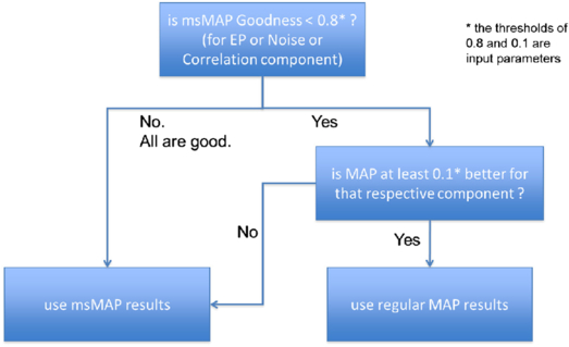
Fig. 12. Logic flow of the vetting process, which decides whether the regular MAP or msMAP fit is used. Includes a selection bias of 0.1 towards msMAP.
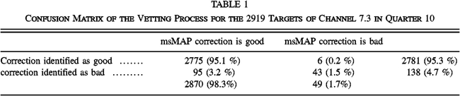
By manual validation of the vetting results, we found that almost all of the bad corrections—about 90%—are successfully detected (using the threshold parameters shown in Fig. 12), in which case PDC reverts back to the regular PDC-MAP correction. The confusion matrix of this vetting process is shown in Table 1 for the 2919 targets of channel 7.3 in quarter 10. Spot tests of other channels and quarters gave similar numbers. With this process, the number of bad corrections is reduced to only a handful (≈0.2%) per channel. For false negatives that revert to regular MAP but for which the msMAP fit is actually good, we find the regular MAP fit is generally good as well, and no harm is done reverting to regular MAP. It is interesting that a large fraction of the targets for which regular MAP performs better than msMAP are highly variable targets. For such targets, msMAP has a tendency to either attenuate the stellar signals or introduce some high-frequency noise. These same targets are precisely the ones the original MAP method (Smith et al. 2012) was designed to correct.
 |
4.2. Goodness Metric: Earth-points
The PDC “goodness metric” previously had three components, which try to quantify the correction performance for each target with regard to (1) residual correlations, (2) preservation of stellar variability, and (3) injection of noise (Stumpe et al. 2012). Motivated by the occasional residual systematic errors for the Earth-point recoveries in PDC-MAP, we have added a fourth component to the goodness metric, which quantifies how well the thermal transients after an Earth-point have been corrected. As with the original three components, we expect this goodness metric component to represent a coarse estimate of the correction quality, rather than a perfectly accurate quantification of the correction performance (which in fact would require the ground-truth light curves). In particular, the goodness metric should help to achieve four goals:
- 1.For each light curve (e.g., processed with both regular MAP and msMAP), to decide which of two possible corrections is more likely to be the better correction.
- 2.For each module output, decide which set of PDC parameters on average produces better results.
- 3.To detect cases where the correction of a target was very poor, so that the respective target can be corrected differently or investigated further.
- 4.To give users of Kepler data an estimate of the quality of the PDC correction for any particular light curve.
Because the thermal transients after an Earth-point roughly follow an exponential shape, we base the calculation of this component on the strength of the exponential character of the light curve in this region. For that purpose, we preprocess the light curve by normalizing it with its median, and performing a simple linear detrending. Then a nonlinear least-squares fit is used to fit an exponential function f(t) = a· exp(b·t) (where a and b are fit parameters) to the recovery window after the Earth-point, defined as the 150 cadences after an Earth-point gap. We use the curvature of the fitted exponential, calculated by the average of its second derivative in the recovery region,  , to quantify the strength of the exponential character. As with the other goodness metric components, the goodness shall be expressed as a value in the interval [0,1), which we achieve by the regularization

where γ is a weighting parameter to adjust the relative emphasis of this component in the total goodness metric G, which is the geometric mean of the four components for residual correlations (GC), noise (GN), stellar variability (GV), and Earth-point recoveries (GEP):

We also tried other metrics to quantify the Earth-point correction, including measuring the deviation of the 150 cadences window after an Earth-point from an autoregressive estimate of this window, and a similar approach to the current one but where we in addition compare to an exponential fit of the region before the Earth-point gap and after the recovery window for reference. Out of the different metrics we tried, the current one is most in line with the perceived correction quality found upon manual investigation. For a detailed explanation and derivation of the goodness metric in PDC, see Stumpe et al. (2012).
4.3. Edge Effect Mitigation
An essential step in computing the wavelet transform of a discrete time series is circular convolution with a scaling filter (Percival & Walden 2000). Wrapping the signal around from the end to the beginning gives rise to undesirable “edge effects” at the boundaries, when there is discontinuity between the first and last parts of the time series. One way to mitigate the edge effects is to extend the time series by reflection, i.e., to append a time-reversed copy of the time series at its right end (Percival & Walden 2000). This ensures continuity, but it does tend to form cusps at the boundary, which also give rise to edge effects. Another extension method is zero-padding, adding zeros at the end of the signal to pad its length (Jensen & la Cour-Harbo 2000). Zero-padding introduces edge effects because of the discontinuity between the ends of the signal and the zeros. When extension methods are used, the time series of wavelet coefficients and of the multiresolution analysis at each scale are subsequently truncated at the boundaries of the original time series.
Another concern regarding edge effects is their temporal extent. When a discrete time series is transformed to the wavelet domain, wavelet coefficients near the boundaries are unreliable, since they are influenced by extrapolated data (if an extension method is used) or by wrap-around (if there is no extension). There is a “zone of influence” in the timeseries of wavelet coefficients at each scale near the boundaries, whose temporal extent increases with scale and also with the length of the wavelet filter (Percival & Walden 2000). Wavelet coefficients at the largest scales are the most affected. The size of the zone of influence at all scales is reduced by using a shorter wavelet filter. We are currently using a Daubechies wavelet with a filter of length 12, which seems to adequately reduce the zone of influence.
We experimented with several extension methods to gauge their effectiveness in edge effect mitigation. We sought a method that would smoothly stitch together the signal and its extensions without the discontinuities and cusps which can give rise to severe edge effects. The method we settled on, which achieves this goal in most cases, involves extending the flux time series at each boundary using a sign-inverted, time-reversed copy of itself, and is explained in detail below.
Matching up the extrapolated signal at the boundaries when the original signal contains an appreciable amount of noise or high-frequency variability introduced an added complication. We addressed the problem by estimating the flux-level at each boundary by low-pass filtering the 500 nearest cadences via linear interpolation. The right and left flux extensions are shifted vertically by the appropriate offsets so that they will match the estimated input flux at the boundaries. This makes the flux extension relatively robust to high-frequency variation or noise in the signal.
The extensions at the left and right boundaries are

and

where F(t) is the flux time series, t1 and t2 are its left and right boundaries, T is the length of the flux time series, G(t) is the reflected version of F,  is the interpolated estimate of F(t1), and r(t) = (t - t1)/(t2 - t1) is a linear ramp from 0 to 1 over the domain of the flux time series. The value of L at its right boundary (where it is to be stitched to the left boundary of the input flux) is
  . Similarly, for R,
  is the interpolated estimate of F(t2) and the value of R at its left boundary (where it is to be stitched to the right boundary of the input flux) is
  . See Figure 13 for an example of the flux extension and subsequent band 1 light curve. Notice that the edges of the band 1 curve are well behaved.
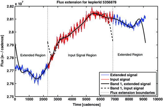
Fig. 13. Edge effect mitigation showing the original light curve, the Band 1 light curve without extended regions, and then the edge effect mitigation extensions and the subsequent Band 1 light curve when utilizing the edge extensions. The Band 1 light curve with edge extensions is clearly well behaved at the light-curve edges.
4.4. Application to Short-Cadence Data
The primary mission for Kepler is detection of Earth-like planets, and so work on the pipeline emphasises long-cadence data. However, short-cadence PDC processed data (at 59 s cadence) is also provided to the users. The principal issue with applying the MAP technique to short-cadence data is the limited number of targets per module output. No more than 512 short-cadence targets are collected at any time and are spread over the entire field of view so the number of short-cadence targets per channel is small, and at most about a dozen. A dozen is too small of a sample for the prior PDF or basis vectors to be properly formulated. However, all short-cadence targets are also long-cadence targets, and so priors are already developed for all short-cadence targets. A simple way to extend MAP to short-cadence data is to use the basis vectors interpolated from long cadence and also the long-cadence fit coefficients as the prior. A future paper will describe the algorithm in detail.
5. Performance Evaluation
With the presented multiscale extension to PDC-MAP, we observe a significant improvement in correction quality as compared to the previous version of PDC-MAP. In particular, the two main deficiencies of PDC-MAP, residual systematic errors and noise injection, are improved in msMAP.
Figure 14 shows several example cases of light curves where regular MAP did not perform an optimal correction, and which show a substantially better correction with the new msMAP. Panels A and B show the initially discussed example from Figure 1. Note that we have deliberately picked cases where the regular PDC-MAP did not perform as well, which as a reminder, is only about every fifth light curve. In the other cases, the corrected time series of regular MAP and msMAP are usually very similar or almost identical.
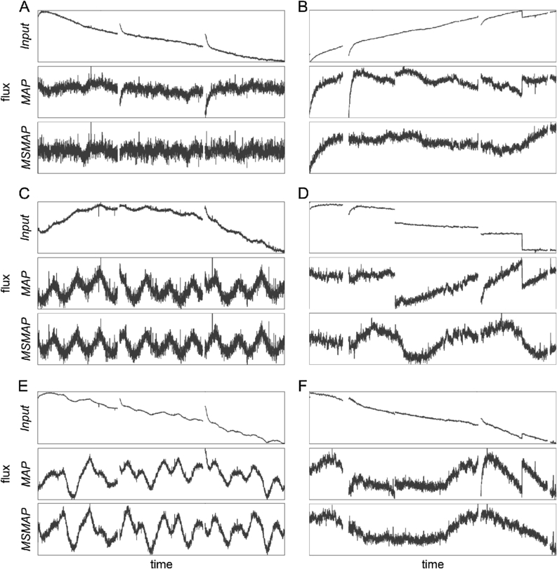
Fig. 14. Examples of msMAP correction performance improvements. The top row in each panel shows the PDC input time series, the middle row the PDC-MAP corrected time series, and the bottom row the msMAP corrected time series. Vertical scales are rescaled between panels to show detail. Panels (a), (c), and (e) show examples with regular data quality (Q10 data), and panels (b), (d), and (f) show cases with very strong systematic errors (Q2 data). The examples in panel (a) and (b) are the same ones as in Fig. 1.
The PDC goodness metric is invaluable in comparing cotrending methods. Here we can use it to compare the performance of a regular MAP run and a new multiscale MAP run. Figure 15 shows the performance of regular MAP versus multiscale MAP for three goodness components: (1) residual correlation, (2) injected noise, and (3) Earth-point recovery removal. These figures are for Quarter 10 module output 2.1 data. Goodness values are plotted as a “cumulative distribution function”, where the horizontal axis gives the goodness value and the vertical axis gives the percent of targets with this goodness or above. The goodness metric is calibrated such that 0.8 or above is considered a “good” correction. There is a clear performance gain in the residual correlation and Earth point components. There is a modest overall performance gain for the noise injection, and the “tail” of targets with noise goodness below 0.8 is reduced by over half. The stellar preservation goodness component does not change substantially, and is not shown in the figure. The fraction of targets with residual correlation (defined by a correlation goodness below 0.8) has been reduced from about 20% down to near zero. The fraction of targets with residual Earth-point recoveries has been reduced from about 40% to 20%.
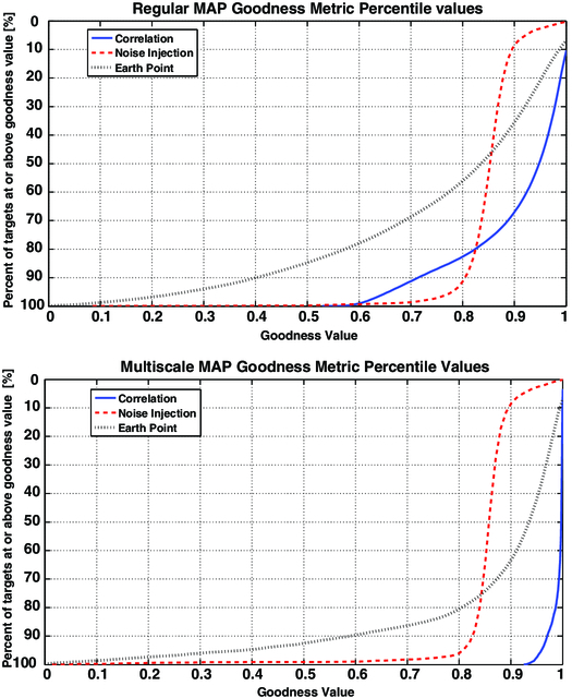
Fig. 15. Comparison of three of the goodness metric components between regular MAP and multiscale MAP. Top: Regular MAP. Bottom: Multiscale MAP.
6. Outlook
One remaining issue is that the Earth-point recoveries have a very strong signal on the order of 150 cadences, which is the same scale as the oscillations from the 3 day reaction wheel desaturation cycle (see Figs. 1b and 1c in Stumpe et al. [2012] for illustrations of these errors). Consequently, these two systematic errors can not be separated based on their characteristic scale. This is generally not a serious problem, but it does lead to one of those two errors not being perfectly corrected in some cases. One option to improve this situation is to explicitly add either of these signals as an additional basis vector. On first sight, the blatant artifact from the Earth-point recoveries might seem like a good candidate to model with a simple exponential following the monthly Earth-point gap. However, their magnitude and shape can vary significantly between light curves, and therefore injecting an artificial basis vector for the whole set of light curves of one CCD channel would likely be nonideal. Another choice would be to add a basis vector for the rather subtle 3 day reaction wheel desaturation cycle, but the resulting trend is not quite periodic or highly regular, since its strength varies from the beginning to end of each quarter. One of the core principles of PDC-MAP has so far been to not use manually designed signals for the basis vectors, but rather to generate them solely from the light-curve data. However, augmentation to provide explicit known trends might prove useful and could be investigated in future work. There is also the option to perform the entire MAP fit in the transformed wavelet domain whereas we currently transform back into the time domain after band-splitting. This may allow us to cleanly separate the reaction wheel desaturation from the Earth-point recoveries.
We would also desire to get a proper MAP fit working for the shortest and longest bands. There is no fundamental reason we cannot or should not. For the longest band the principal obstacles are resolving the issue with wavelet artifacts (see § 3.3) and obtaining better long-period priors. For the shortest band, we have found the flux to mainly contain high-frequency noise. However, some systematic spikes are visible. These are mostly due to Argabrightenings and spurious spikes from the read-out electronics and could be removed with proper basis vectors. A denoising technique could extract these signals from the underlying noise.
Perhaps the most promising candidate for further improvement is the generation of better priors for the MAP-fit. As has been discussed for the original version of PDC-MAP (Smith et al. 2012) and again in this work (see § 4.1), bad priors can sometimes lead to a very low correction quality. This problem is mitigated here in the new msMAP, because cases of poor performance are identified automatically by the goodness metric quality control and the better of the two corrections (msMAP or regular MAP) is used. However, even better would be to avoid these corrections in the first place. Furthermore, better priors would most likely also solve the problem where using a MAP-fit in the longest-scale band can lead to an artifact. To that end, a detailed investigation of the cause of bad priors and their remediation in PDC-MAP is being undertaken. Improvements to the priors will be presented in a future paper.
7. Summary And Conclusion
We have developed the next generation of the Kepler presearch data conditioning module, which is a central part of the Kepler data processing pipeline and is tasked with correcting systematic errors in the light curves. Our new approach, using wavelet-based bandsplitting to decouple errors on different scales and perform a multiscale correction, significantly improves the quality of the light curves. In particular, the two main problems of the previous version of PDC-MAP, residual systematic errors and injection of high-frequency noise, are improved in the new Multiscale PDC-MAP. In a sense, the correction characteristics of msMAP can be regarded as the best of both worlds from the first version of PDC-LS (Twicken et al. 2010a) and the original PDC-MAP (Smith et al. 2012). The former only rarely exhibited residual systematic errors in the light curves, but was prone to overfitting and removal of astrophysical features. The latter represented a milestone improvement and was not sensitive to overfitting at all, but it sometimes was too conservative in preserving residual systematics in the light curves. The performance of our new msMAP can be tuned to both of these extremes by setting the parameters accordingly, in particular the number of bands. Between these extremes, we found that there is an optimum parameter set (i.e., 3 or 4 bands) that delivers excellent correction of systematic errors without removal of astrophysical signals and without injection of high-frequency noise. Further, our extensive testing of the parameter range showed that this optimum parameter set is sufficiently broad and robust and that the excellent correction quality can be achieved for almost all CCD channels and data quarters without the need for individual fine-tuning of the parameters for each situation. Rare cases where the multiscale correction fails are caught by an automatic quality control process via the PDC goodness metric, which has been extended by a fourth component to assess the correction of the thermal transients after Earth-points or similar data gaps. In summary, msMAP is capable of producing error-corrected light curves of unprecedented quality and we expect that users of the Kepler data will hugely benefit from these improvements for both the study of stellar astrophysics as well as the search for extrasolar planets.
Funding for this Discovery Mission is provided by NASA’s Science Mission Directorate. We thank the thousands of people whose efforts made Kepler’s grand voyage of discovery possible. We especially want to thank the Kepler Science Operation Center and Science Office staff who design, build, and operate the Kepler Data Analysis Pipeline and for putting their hearts into this endeavor.
Facilities: Kepler.
Footnotes
- 5
In simple aperture photometry, the brightness of a star in a given frame is measured by summing up only the pixel values in the core image that increase SNR.
- 6
See http://stdatu.stsci.edu/kepler/.
- 7
As of September 2013, Kepler management has announced the end of fine-point data collection with three or more reaction wheels.
- 8
It should be noted that the current Kepler pipeline architecture does not allow for specific parameters for individual channels but only for individual quarters where all channels in each quarter use the same parameters.
- 9
Details of stellar preservation in PDC is to be published in a forthcoming paper.