
ABSTRACT
We present fitted UBVRI - ZY and u′ g′ r′ i′ z′ magnitudes, spectral types, and distances for 2.4 million stars, derived from synthetic photometry of a library spectrum that best matches the Tycho2 BT VT, NOMAD RN, and 2MASS JHK2/S catalog magnitudes. We present similarly synthesized multifilter magnitudes, types, and distances for 4.8 million stars with 2MASS and SDSS photometry to g < 16 within the Sloan survey region, for Landolt and Sloan primary standards, and for Sloan northern (photometric telescope) and southern secondary standards. The synthetic magnitude zero points for BT VT, UBVRI, ZV YV, JHK2/S, JHKMKO, Stromgren uvby, Sloan u′ g′ r′ i′ z′, and ugriz are calibrated on 20 CALSPEC spectrophotometric standards. The UBVRI and ugriz zero points have dispersions of 1–3%, for standards covering a range of color from -0.3 < V - I < 4.6; those for other filters are in the range of 2–5%. The spectrally matched fits to Tycho2 stars provide estimated 1σ errors per star of ∼0.2, 0.15, 0.12, 0.10, and 0.08 mag, respectively, in either UBVRI or u′ g′ r′ i′ z′; those for at least 70% of the SDSS survey region to g < 16 have estimated 1σ errors per star of ∼0.2, 0.06, 0.04, 0.04, and 0.05 in u′ g′ r′ i′ z′ or UBVRI. The density of Tycho2 stars, averaging about 60 stars per square degree, provides sufficient stars to enable automatic flux calibrations for most digital images with fields of view of 0.5° or more. Using several such standards per field, automatic flux calibration can be achieved to a few percent in any filter, at any air mass, in most workable observing conditions, to facilitate intercomparison of data from different sites, telescopes, and instruments.
1. INTRODUCTION
Reliable flux calibration is important for accurate photometry and to compare observations taken by different observers at different times or different sites with different equipment and possibly different filter bandpasses.
Ground-based optical calibration is traditionally achieved by observing both standard stars and at least some stars in the field of interest, with the same equipment, during periods known to be photometric. In principle, this permits calibration of program stars on a standard photometric system to better than 1%, but in practice, filter and instrumental mismatches, atmospheric, and other variations during this process often limit effective calibration to 2% or worse.
Internal relative flux calibration of single or repeated data sets are routinely achieved to 0.2% or better, including during nonphotometric conditions, by reference to nonvariable stars in the observed field. But significant questions arise about effective cross calibration of observations from different epochs. The situation is particularly complicated for time-domain science, where multiple sites, telescope apertures, filters, and sets of instrumentation become involved, or when time constraints or observing conditions preclude traditional calibrations. Offsets between otherwise very accurate data sets can be much larger than expected. This can introduce significant uncertainty in multiobservation analysis or obscure real variations.
Cross comparisons can be facilitated by parallel wide-field observations along the line of sight to each image, as in the Canada-France-Hawaii Telescope (CFHT) SkyProbe1 facility (Cuillandre et al.2004) or other context camera systems. But having multifilter standards within each digital image offers many simplifying advantages. The ideal scenario for calibration of optical imaging data would be if there were all-sky stars of adequately known brightness on standard photometric systems and that were present in sufficient numbers to provide a few in every digital image.
Precursors to such standards include:
- 1.
- 2.
- 3.The U.S. Naval Observatory (USNO) Naval Observatory Merged Astrometric Dataset4 (NOMAD) catalog (Zacharias et al.2004), which contains over one billion stars covering the whole sky. It is often used for automatic astrometric fits and has calibrated photographic RN -band photometry (on the Landolt system), with a dispersion of about 0.25 mag.
The Tycho2 catalog (Høg et al.2000) provides a consistent set of all-sky optical standards, observed with the Hipparcos 5 satellite. It provides ∼2.5 million stars to about 13.5 and 12.5 mag in BT and VT filters. While this catalog contains less than 1% of the stars in the 2MASS catalog and has large photometric errors at the faint end, it forms the basis (along with 2MASS and NOMAD) for an effective and consistent all-sky photometric catalog that can be used by many optical telescopes to achieve reasonable automatic flux calibration.
The average density of Tycho2 stars varies from ∼150 stars per square degree at Galactic latitude b = 0° through ∼50 stars per square degree at |b| = 30° to ∼25 stars per square degree at |b| = 90° (Høg et al.2000), so it is typically possible to find 5–15 Tycho2 stars within a 30′ field of view. These numbers obviously decrease for smaller fields of view and become uninteresting for fields of view much smaller than 15′. The footprints in equatorial coordinates of several catalogs discussed here are shown in Figure 1.
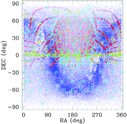
Fig. 1.— The footprint in equatorial coordinates of the various catalogs is discussed here. The Tycho2 catalog (blue dots) covers the whole sky to BT ∼ 13.5 mag. The Sloan survey (red dots) covers less area, but to a much fainter limiting magnitude, shown here to g < 16 mag. The Landolt primary standards are marked with green crosses; the Sloan primary standards are marked with yellow circles; the southern Sloan secondary standards are marked with cyan squares, where each square represents many standards; and the northern SDSS-PT stars are marked with cyan dots.
Ofek (2008) described how to produce synthetic g′ r′ i′ z′ magnitudes for about 1.6 million Tycho2 stars brighter than 12 mag in VT and 13 mag in BT. The present paper extends this to 2.4 million Tycho2 stars, with synthetic magnitudes on both the Landolt and Sloan standard photometric systems, and to other filter systems calibrated here, such as Stromgren and UKIRT ZY and JHKMKO.6 The methodology permits post facto extrapolation to other filter systems of interest and can be applied to future all-sky catalogs of greater depth and accuracy.
In § 2 we describe our calculations of synthetic magnitudes and fluxes from flux calibrated digital spectra.
In § 3 we describe the zero-point calibration of our synthetic photometry against the de facto standard: 20 spectrophotometric standards with photometric data and covering a significant color range, taken from the Hubble Space Telescope (HST) CALSPECproject.7
In § 4 we describe the spectral matching library and calibrated magnitudes in different filter systems: BT VT, UBVRI, J2 H2 K2/S, UKIRT ZY and JHKMKO, Stromgren uvby, and Sloan filter sets, both primed and unprimed system bandpasses.
In § 5 we describe the spectral matching process, χ2 optimization, and distance constraints.
In § 6 we illustrate the spectral matching and flux fitting methodology, with results fitted with different combinations of optical and infrared colors for Landolt and Sloan primary standards.
In § 7 we further illustrate the strengths and limitations of the spectral fitting method with ∼16,000 southern Sloan standards (Smith et al.2005) and with ∼1 million SDSS photometric telescope (PT) secondary patch standards (Tucker et al.2006; Davenport et al.2007) with 2MASS magnitudes; ∼11,000 of those also have Tycho2 BT VT magnitudes and NOMAD RN magnitudes.
In § 8 we describe online catalogs with fitted types, distances, and magnitudes in UBVRI - ZY and u′ g′ r′ i′ z′ for: (1) Landolt and Sloan primary standards, (2) Sloan secondary north and south standards, (3) 2.4 million Tycho2 stars, and (4) 4.8 million stars within the Sloan survey region to g < 16.
2. SYNTHETIC PHOTOMETRY
Bessell (2005) describes the preferred method for convolving an F(λ) digital spectrum with filter/system bandpass sensitivity functions to obtain synthetic magnitudes that take account of the photon-counting nature of modern detectors,
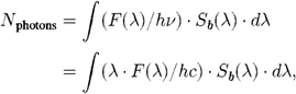
which can be normalized by the filter/system bandpass to form the weighted mean photon flux density:

As Bessell (2005) notes, this weights the fluxes by the wavelength and shifts the effective wavelength of the bandpass to the red. This is the basic convolution methodology used in the HST Synphot8 package. From the Synphot User’s Guide we can form

where the numerical factor for the nominal F(λ) at V = 0 brings the resultant magnitudes close to standard values.9 Additionally, as discussed in the Principles of Calibration section of the Synphot User’s Guide, we can form the effective wavelength,
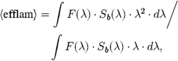
and the source-independent pivot wavelength,
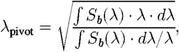
and form a magnitude system based on F(ν) as

where the numeric constant, as derived in Sirianni et al. (2005), has the advantage of bringing magν close to the AB79 system of Oke & Gunn (1983). The bandpass zero points in equation (1) are to be determined.
Pickles (1998) adopted a different approach based on mean flux per frequency in the bandpass 〈F(ν)〉. The differences between this and the Synphot methods for calculating magnitudes are typically of the order of 0.02 to 0.04 mag over most of the color range, but for very red stars with nonsmooth spectra can become as large as 0.1 mag in R, which has an extended red tail. Importantly, the Synphot approach produces less zero-point dispersion for stars covering a wide range of type and color, and it is adopted here.
3. FILTERS AND ZERO POINTS BASED ON SPECTROPHOTOMETRIC STANDARDS
All the filter bands discussed here (except the medium-band Stromgren filters) are illustrated in Figure 2. Only the wavelength coverage and, particularly, the shape of the system bandpass matter, not the height, which is taken out in the filter normalization.
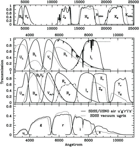
Fig. 2.— The filters discussed here are illustrated. In the first panel the Tycho2 BT VT filter system transmissions are taken from Maiz Apellániz (2006) and overplotted (dotted lines) in the third panel for convenient reference. The 2MASS J2 H2 K2/S system total response curves are from the IPAC Web site; the JHKMKO filter transmission curves (dotted) are from Tokunaga et al. (2002). In the second panel the Landolt UL BL VL RL IL transmission curves for the filters alone are shown (dotted lines; Landolt 1992a); their system response including typical atmosphere and detector QE are shown (solid lines; Cohen et al. 2003a). In the third panel the synthetic UM BM VM filters are from Maiz Apellániz (2006) (VM; dashed line); the VC RC IC curves are from Bessell (1979), and the ZV YV (solid) curves are from the UKIRT/VISTA collaboration. The PTF Mould-type Rp system response is also illustrated, as are the LCOGT ZS YE system responses (dotted lines) discussed in § 6.1.1. In the bottom panel the Sloan survey system bandpasses are shown for both the unprimed survey imaging bandpasses (dotted lines), where the filter interference red edges move bluer in the vacuum of the survey camera, and primed bandpasses used in air for PT and southern standard observations (u′ g′ r′ i′ z′; solid lines); they are from the JHU skyservice and the USNO Fermi National Accelerator Laboratory Web sites.
Our approach is similar to that presented by Holberg & Bergeron (2006) but deliberately attempts to calibrate a large number of filters with standards covering a wide range of color and spectral type. The small zero-point dispersions achieved here demonstrate the validity of this approach over a wide variety of spectral types and colors. They reinforce the advances that have been made in accurate flux calibration, as the result of careful work by Bohlin (1996), Colina & Bohlin (1997), Bohlin et al. (2001), and Bohlin (2010).
3.1. CALSPEC Standards
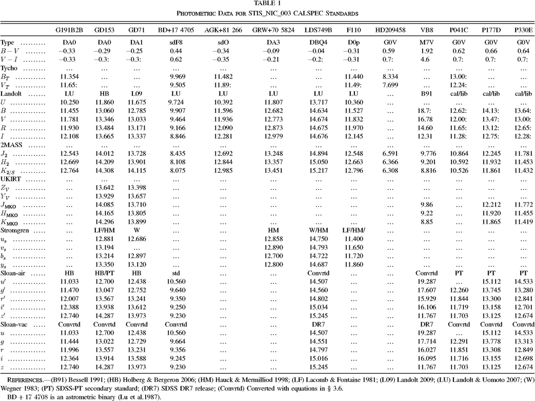
There are 13 standards with Space Telescope Imaging Spectrograph (STIS) NIC3 calibrated spectrophotometry covering 0.1 to 2.5 μ, which include the latest HST CALSPEC calibration enhancements and the 2010 corrections to STIS gain settings. The spectra are mainly of white dwarfs, but include four G dwarfs and VB8 (Luyten half-second, LHS 429, a late-M dwarf) so provide significant color range: -0.3 < V - I < 4.6.
There are two K giants (KF08T3 and KF06T1) with low reddening that were observed with NICMOS to provide Infrared Array Camera (IRAC) calibration (Reach et al.2005). There is little optical standard photometry for these two K giants, so they are only included in the 2MASS JHK2/S zero-point averages, but optical colors estimated from their types are shown to be consistent with the derived optical zero points.
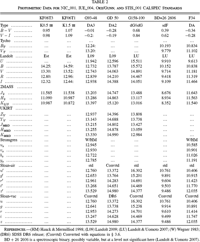
There are three additional CALSPEC white dwarfs with coverage to ∼1 μ (G93-48, GD 50, and Feige34) and two subdwarfs (G158-100 and BD + 26 2606) observed by Oke (1990) and Oke & Gunn (1983) for which fairly extensive photometric data are available in the literature. The latter five spectra calibrated from the uv to ∼1 μ were extended to 2.5 μ for illustrative purposes. Their synthetic infrared magnitudes are computed and shown for comparison, but only their optical zero points are combined in the averages.
3.2. Standard Catalog Magnitudes
The matching catalog photometric data for CALSPEC standards come from the following:
- 1.Tycho2 catalog for BT VT.
- 2.2MASS catalog for J2 H2 K2/S.
- 3.
- 4.Bessell (1991) for optical and infrared photometry of VB8 (M7V).
- 5.UKIRT standards listed on the Joint Astronomy Center’s UKIRT World Wide Web site10 for JHKMKO and their Wide Field Camera (WFCAM) ZYMKO data.
- 6.
All the preceding catalog data are on the Vega system, where the magnitudes of Vega are nominally zero in all bands.
Sloan catalog data on the AB system are from Smith et al. (2002) for primary standards; from the SDSS-PT catalog (Tucker et al.2006; Davenport et al.2007) for southern SDSS standards (Smith et al.2005); from the SDSS Data Release 7 (DR7) database11 for LDS749B, VB8, and GD50; and in two cases (G191-B2B and GD71) from Holberg & Bergeron (2006) for u′ g′ r′ i′ z′ magnitudes.
Additional UBVRI and ugriz photometric data for GD153 (DA0) are from Holberg & Bergeron (2006). Additional BV data for P041C, P177D, P330E (G0V), KF08T3 (K0.5 III), and KF06T1 (K1.5 III) are from the CALSPEC Web site.
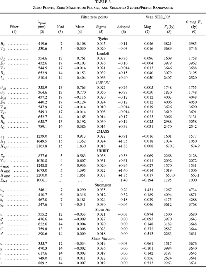
Photometric data for the CALSPEC standards are summarized in Tables 1 and 2. Table 3 summarizes our derived filter bandpass results.
 |
 |
 |
In Table 4 we have computed mean fluxes and synthetic magnitudes by equation (1) in the system bandpasses of all the filters for up to 20 standards that have both accurate digital spectra available from CALSPEC and measured photometry from the literature. Table 4 lists all the digitally measured spectrophotometric data for each spectrum and filter, including average wavelengths 〈λ〉; effective wavelengths 〈efflam〉; pivot wavelengths (which are the same for each star); mean fluxes 〈F(λ)〉, 〈λ.F(λ)〉, and 〈F(ν)〉; and catalog magnitudes from the literature where available, with quoted errors.
For each standard and each filter, magnitudes have been computed via equation (1), and the zero points have been calculated to match synthetic to observed magnitudes. The calculated values are listed in Table 5.
3.3. Zero-Point Means and Dispersions
In Table 3 we summarize for each filter the synthesized pivot wavelengths, zero-point means and dispersions, adopted zero points, measured magnitudes and fluxes of the STIS_005 CALSPEC spectrum of Vega, and our derived values of 〈F(ν)〉 for 0 mag in all filters.
Figure 3 shows the filter bands overplotted on the STIS_005 CALSPEC spectrum of Vega, plotted as F(ν) vs. wavelength. The spectrum illustrates the nominal zero-magnitude definition for filters on the Vega system, and the horizontal line at 3631 Jy illustrates the AB = 0 mag reference. The points show our synthesized Vega magnitudes from column (7) of Table 3, and the error bars show our zero-point ± 2σ dispersion errors from column (5) of Table 3.
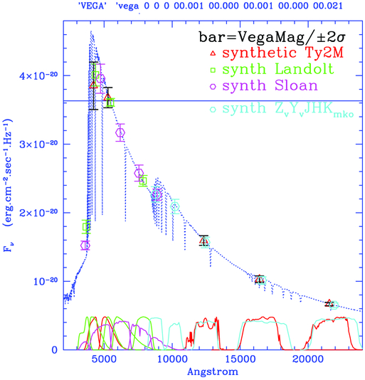
Fig. 3.— Bandpasses, zero points, and synthetic measurements for the CALSPEC spectrum STIS_005 spectrum of Vega (bluedotted-line trace), which defines the nominal zero-magnitude definition for filters on the Vega system. The horizontal line at 3.631 ∗ 10-20 ergs cm-2 s-1 Hz-1 (3631 Jy) illustrates the AB = 0 mag reference. Tycho2/2MASS BT VT JHK2/s bandpasses are indicated by red traces, synthetic flux measurements are red triangles, and zero-point dispersion values about them are error bars in black. All error bars here show ± 2σ zero-point dispersion for better visibility. Adopted Landolt UM BM VC RC IC bandpasses are shown as green traces, synthetic flux measurements are green squares, and zero-point dispersion values are green bars. Sloan u′ g′ r′ i′ z′ bandpasses are shown in magenta, synthetic measurements are magenta circles, and zero-point dispersion values are magenta bars. The UKIRT ZV YV JHKMKO bandpasses are shown as cyan traces, synthetic measurements are cyan circles, and zero-point dispersion values about them are cyan bars.
Some uncertain zero-point values in Table 5 are marked with a colon (xxx:) to indicate they are derived from catalog photometry (in Tables 1, 2, and 4), which is uncertain by 0.1 mag or more. Zero-point values enclosed in parentheses indicate values that are not used to form the final zero points. Either they are photometric estimates, or literature values that are out of range, as discussed in the text. The number of standards included in each filter zero-point calculation ranges from 5 for VT to 17 for B and V.
The 2MASS and SDSS coordinates of VB8 differ by 7.4″, corresponding to the large proper motion (-0.77, -0.87″ yr-1) for this star between the epochs of the two surveys. We obtain good VB8 zero-point fits for BVRI, J2 H2 K2/S and HKMKO and grz, but not for JMKO, u, or i bands (see also § 3.6). There is no U -band photometry for VB8.
3.4. Choice of Landolt Synthetic Filter Bandpasses
For UBVRI we tested several possible synthetic system bandpass profiles from the literature. We have made an empirical choice of the best system bandpass(es) that minimize zero-point scatter in the fitted mean zero points for each filter, over the full color range.
In Table 3, we list zero points for UBVRI using both Landolt (system) filter response functions convolved with a typical atmosphere and detector response (Cohen et al.2003a) and synthetic system bandpasses for UM BM VM from Maiz Apellániz (2006) and VC RC IC from Bessell (1979).
It may seem that the Landolt system response curves would provide the optimum synthetic matches to Landolt photometry, but this is not necessarily the case and is not shown by our results in Table 3 and illustrated in Figure 4.
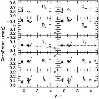
Fig. 4.— Zero points for UL BL VL RL IL (left) and UM BM VC RC IC system bandpasses (right) as a function of standard V - I color. The ordinate scale is set so that vertically higher zero points result in magnitudes that are larger (fainter). Vertical error bars indicate the average and ± 1σ dispersion in each panel. Crosses indicate white dwarfs, and pentagons indicate dwarfs. Three-point crosses indicate the two K giants, which are not included in these zero-point averages or dispersions, as they lack UBVRI photometry. The reddest point corresponding to the M7V VB8 lacks U -band data. The selected UBVRI system profiles on the right minimize zero-point scatter and trend with color.
Both Landolt and Kron-Cousins measurements seek to emulate the original Johnson system for UBV. Both apply calibrating steps in terms of color to their instrumental magnitudes, to bring them into correspondence with standard system values extending back several decades. These steps are summarized in Landolt (2007), for example, and in Landolt (1983, 1992a, 1992b, 2009) to illustrate how equipment changes over time have required slightly different color corrections to maintain integrity with the original system definition. These calibration steps are further reviewed in Sung & Bessell (2000).
Real photometry is done with bandpasses that can vary with evolving instrumentation. We could measure synthetic magnitudes in the Landolt bandpasses and apply color corrections to achieve standard values. But synthetic photometry of flux calibrated spectra has the advantage of being able to select bandpass profiles that minimize dispersion and color effects. We have not attempted to optimize any bandpasses here, but have selected among those available from the literature. For UBVRI, the results in Table 3 indicate that these are best provided by the UM BM VC RC IC bandpasses.
The zero-point dispersions are 0.027, 0.020, 0.008, 0.014, and 0.016 mag for UM BM VC RC IC, respectively, in Table 4, for the full color range from white dwarfs to VB8 (-0.3 < V - I < 4.6). The effective wavelengths vary from 355 to 371 nm, 432 to 472 nm, 542 to 558 nm, 640 to 738 nm, and 785 to 805 nm for UM BM VC RC IC, respectively, between white dwarfs and VB8. Figure 4 illustrates that the selected bands show much less zero-point dispersion than do UL BL VL RL IL, with negligible trend with color. In Figure 4 (and for other zero-point figures) the ordinate is inverted so that zero points that appear vertically higher result in larger (fainter) magnitudes.
This is not a criticism of Landolt system response curves, which enable accurate photometry with appropriate calibration and color corrections, but indicates that the selected UM BM VC RC IC system profiles are best for deriving synthetic spectrophotometry of flux calibrated spectra to properly match Landolt photometry.
The zero-point dispersions for U3 B3 from Azusienis & Straizys (1969) and Buser (1978) are worse, at 0.050 and 0.024 mag, respectively. The dispersion for VM is marginally worse than for VC, where VC has a slightly more elongated red tail than VM.
The zero-point dispersions for UBVRI and ugriz (primed and unprimed) in Table 3, typically closer to 0.02 mag than 0.01 mag, indicate both the accuracy and the limitations of comparing synthetic photometry of well-calibrated spectra with good standard photometry. Tighter fits can be obtained by restricting the selection of comparison stars (for instance, to only WD standards), but such zero points can then be a function of color and lead to synthesized magnitude errors for other stellar types that are much larger than the nominal dispersion for a restricted set of standards.
We are gratified that these comparisons match so well over a large range of color and standard types, confirming the increasing correspondence (currently at the 1–3% level) between spectrophotometric and photometric standards. This sets the basis for enabling synthetic magnitudes of an extended spectral library to be calibrated on standard photometric systems.
3.5. Other Synthetic Filter Zero Points on the Vega System
The system transmission functions for BT VT have been taken from Maiz Apellániz (2006). The zero-point dispersions for BT VT are 0.045 and 0.020, respectively, which are acceptable given the typical errors in the photometric values for fainter stars and several stars included here. There are a total of seven values covering a color range from white dwarfs to G dwarfs for BT, but only five with accurate VT information, with HD209458 (G0V; observed out of planet occultation) being the reddest comparison standard for BT VT.
The filter transmission functions for ZY have been taken from the Vista Web site.12 In what follows we refer to (upper case) ZV YV for these filter bandpasses, where we are using the subscript V to refer to both the Visible and Infrared Survey Telescope for Astronomy (VISTA) and UKIRT Infrared Deep Sky Survey (UKIDSS) consortium and the fact that these are Vega-based magnitudes. The UKIRT WFCAM detector QE is not included in the system bandpass, but, unlike a CCD, it is roughly flat over these wavelengths.13 The dispersions for ZV YV zero points, compared with only five and four UKIRT standards measured with the WFCAM filters, are 0.038 and 0.031 mag, respectively. The YV zero point for G158-100 is suspect, as its CALSPEC spectrum is not well defined at 1 μ. ZV YV zero-point determinations may improve as more photometric standards in common with spectrophotometric standards are measured. The zero-point results and somewhat restricted color ranges for BT VT ZV YV are illustrated in Figure 5.
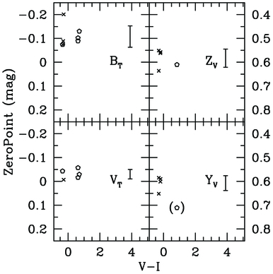
Fig. 5.— Zero points are shown for BT VT (left ordinate) and ZV YV (right ordinate) as a function of standard V - I color, with averages and dispersions as vertical bars. The YV zero point for G158-100 is shown in parentheses but not included in the average. Symbols are as in Fig. 4.
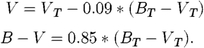
Having a wider color range here for comparison would clearly be advantageous, but there are several mitigating factors. The BT and ZV YV bandpasses are more rectangular in shape than are the B and z bandpasses, for example. They have effective wavelengths that vary less with color and are therefore less susceptible to color effects suffered by filters with extended tails. The ranges of effective wavelengths from white dwarfs to VB8 are 416.3 to 440.4 nm, 524.3 to 543.1 nm, 875.1 to 884.9 nm, and 1018.8 to 1023.2 nm for BT VT ZV YV, respectively. The BT - VT colors derived from our synthesized flux library, Table 6 (see § 4) also follow the standard Tycho2 conversion formulas,14 with standard deviations of less than 0.02 and 0.03 mag, respectively, over a large color range:
Similarly, as shown in § 6.1.1, the synthesized ZV and z′ data fit well over a wide color range, indicating an extended range of validity beyond that illustrated in Figure 5.
The YV data are included because several survey cameras (Panoramic Survey Telescope and Rapid Response System [Pan-STARRS],15 SkyMapper,16 Dark Energy Survey,17 UKIDSS/VISTA,18, and our Las Cumbres Observatory Global Telescope (LCOGT)19 monitoring cameras are using or plan to use a Y filter at ∼1 μm. This is further discussed in § 6.1.1.
The transmission functions of the 2MASS filters, including detector and typical atmosphere, have been taken from the IPAC Web site.20 The zero-point dispersions for J2 H2 K2/S, indicated graphically in Figure 6, are about 0.02 mag, quite comparable with the typical (low) 2MASS errors for these stars, and the zero points show no trend with color.
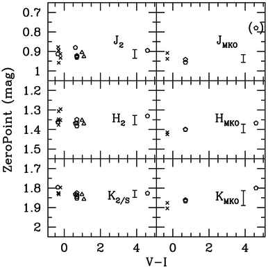
Fig. 6.— Zero points are shown for J2 H2 K2/S (left) and JHKMKO (right) as a function of standard V - I color, with averages and dispersions. Symbols are as in Fig. 4. The K III points (triangles) have been included for JHK2/S. The zero points for JHKMKO show some trend with color, but the JMKO value for VB8 has been excluded due to uncertainty over its magnitude.
The transmission functions for the JHK filters on the Mauna Kea Observatory system have been taken from Tokunaga et al. (2002). Unlike the 2MASS system bandpasses, these do not include detector QE or atmosphere. The zero-point dispersions for JHKMKO are 0.02, 0.02, and 0.04, respectively, for relatively few standards, but they do show trends with color. We indicate the JMKO zero point for VB8 in Figure 6 but, due to uncertainty with its catalog magnitude, we have not included it in the JMKO zero-point average.
The transmission functions for the Stromgren filters (not illustrated) are from Maiz Apellániz (2006). The zero points derived in Table 3 are -0.29 ± 0.04, -0.32 ± 0.01, -0.18 ± 0.02, and -0.04 ± 0.03 for Stromgren uvby, respectively. These are averaged over seven CALSPEC white dwarfs for which Stromgren photometry was found in the literature. The validity of these zero points for redder stars is not demonstrated, but the effective wavelength variations with color are small for medium-band filters with rectangular profiles, so zero-point variations with color should not be large for the Stromgren filter bandpasses. Figure 7 illustrates the zero points for Sloan primed and unprimed filters, discussed in § 3.6.
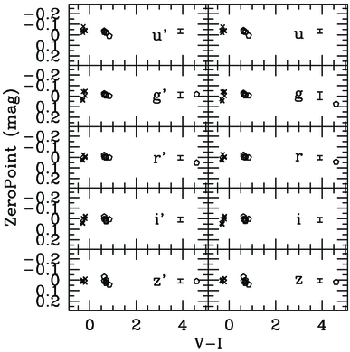
Fig. 7.— Zero points are shown for u′ g′ r′ i′ z′ (left) and ugriz (right) as a function of standard V - I color, with averages and dispersions. VB8 is present in the grz plots, but has been omitted in the ui plots. Symbols are as in Fig. 4.
3.5.1. Mould R Band
The Rp filter system profile shown in Figure 2 is a Mould R -band interference filter with rectangular profile, of the type used at many observatories to measure R on the Landolt system. In this case it is the CFH12K 7603 filter originally from CFHT21 and now used Palomar Transient Factory.22 The Rp system profile includes the CCD response and atmospheric transmission appropriate to 1.7 km and air mass 1.3, although both of these are roughly flat in this region. The zero point (Table 3) for this filter profile excludes VB8, since the lack of a red tail results in magnitudes that are too faint for stars redder than R - I > 0.6.
Figure 8 shows (upper panel) the comparison of Rp - RC with Landolt R - I color, which results in a tight two-segment curved fit. The lower two panels show Rp - RC and Rp - r′ against the Sloan r′ - i′ color, both of which show reasonable two-segment linear fits, confirming that rectangular-shaped Mould R observations can be reliably converted to standard R magnitudes:
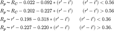
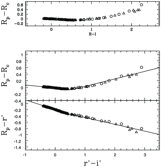
Fig. 8.— Upper panel: Rp - RC color plotted against the Landolt R - I color. The fit is tight, but curved in both segments. Dwarfs are indicated as pentagons, subgiants are squares, giants are triangles, and supergiants are crosses. Lower panels: Rp - RC and Rp - r′ colors vs. Sloan r′ - i′. Symbols are as in the top panel. In these cases there are good two-segment straight-line fits.
3.5.2. NOMAD R Band
The USNO NOMAD catalog (Zacharias et al.2004) contains BVR and JHK data for many stars. The NOMAD BV data for brighter stars are typically derived from Tycho2 BT VT using standard conversion formulas referenced in § 3.5. It is possible to compare these converted values with synthesized BV magnitudes, but it is better and more accurate to compare as we have done with the Tycho2 BT VT values: directly with their synthesized values in the BT VT system bandpasses. The NOMAD JHK magnitudes are from 2MASS, so do not provide additional information.
The NOMAD R -band data are derived from the USNO-B catalog, which was photometrically calibrated against Tycho2 stars at the bright end, and two fainter catalogs, as described in Monet et al. (2003), with a typical standard deviation of 0.25 mag.
Figure 9 illustrates our comparison of NOMAD R -band data against Landolt standards and 16 CALSPEC standards. The data are plotted as the differences RNomad - RLandolt vs. RLandolt. A 3σ clip has been applied that excludes about 10 stars plotted as black crosses, but retains more than 98% plotted as red crosses. The dashed-line histogram of all the stars shows the distribution of these differences plotted with increasing number to the right against the magnitude delta on the ordinate. This shows a good one-to-one fit, with zero mean offset and a 1σ dispersion of 0.25 mag for sigma-clipped Landolt stars. The equivalent dispersion is 0.17 mag for the CALSPEC stars, excluding VB8. The location of the red M dwarf VB8 is indicated: the photographic R band, like the preceding Mould-type R band, lacks the red tail of the Kron/Cousins/Landolt R filter, so measures magnitudes that are too faint for extremely red stars, when the flux is rising rapidly through the bandpass.
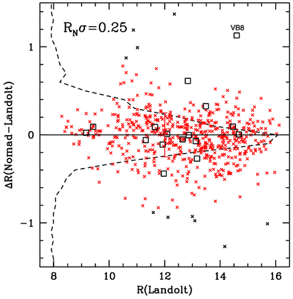
Fig. 9.— Comparison of NOMAD and Landolt R -band data plotted as the difference RN - RLandolt vs. RLandolt (crosses) and CALSPEC standards (squares); VB8 is identified. Black crosses show about 10 points rejected by a 3σ clip, and red crosses show those remaining. The resulting 1σ dispersion of 0.25 mag is indicated. The dashed-line histogram of all the stars shows the distribution of these differences plotted with increasing number to the right against the magnitude delta on the ordinate.
It would be preferable to compare digitized photographic R magnitudes with synthesized values in the appropriate system bandpass, but this is clearly impossible and probably would not improve this calibration. The NOMAD R -band calibration is linear over a significant magnitude range and the dispersion is roughly constant with magnitude, probably indicating the difficulties of measuring digitized plates, rather than any linearity or systemic calibration issues.
In § 5 we include the NOMAD RN -band data together with Tycho2 and 2MASS magnitudes to provide six-band spectral matching of the Tycho2 stars, where the catalog RN is matched to our synthesized RC magnitude, because inclusion does improve the fits slightly over just Tycho2/2MASS fits. We adopt a photometric error of 0.25 mag for all NOMAD RN magnitudes.
3.6. Sloan Filters on the AB System
The system transmission functions of the unprimed ugriz filters used in the imaging camera, including typical atmosphere at 1.3 air masses and detector response, have been taken from the SDSS Web site.23 Those for the primed u′ g′ r′ i′ z′ filters used for standard observations have been taken from the USNO Web site24 for 1.3 air masses.
In order to compute zero points for the imaging survey (unprimed) Sloan bandpasses ugriz, we computed conversion relations between the primed and unprimed Sloan system values by comparing synthetic magnitudes of digital library spectra from Pickles (1998), as listed in Table 6 (§ 4). This approach avoids many complexities detailed in Tucker et al. (2006) and Davenport et al. (2007), but produces tight correspondence between synthetically derived Sloan primed and unprimed magnitudes, over a wide color range.
With the exception of two zero-point adjustments for g and r, these relations are identical to those listed on the SDSS site25 and are summarized here:
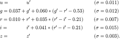
These relations were used to convert SDSS standard values on the primed system to unprimed values (and vice versa when only DR7 data were available: e.g., for LDS 749B, P177D, P330E, and GD 50) then compared with synthetic magnitudes computed in the unprimed bandpasses to derive their zero points and dispersions.
The SDSS DR7 u -band data for VB8 appears too bright, likely because of the known red leak. The DR7 i -band magnitude is close to the r -band magnitude and appears too faint for such a red star. As mentioned in § 3.2 we have omitted the u and i -band data for VB8 from our zero-point averages.
The zero-point dispersions for u′ g′ r′ i′ z′ and ugriz listed in Table 3 are about 0.02 mag (slightly worse for the g band) for up to 14 standards covering a wide color range.
There is little evidence for nonzero zero points in griz; they are zero to within our measured dispersions, and we have chosen to set them to zero. We find zero points for both u′ and u of -0.03 ± 0.02 mag. The zero-point results for u′ g′ r′ i′ z′ and ugriz are illustrated in Figure 7 and show essentially no trend with color.
We find that synthetic spectrophotometry with the published Sloan system transmission functions (u′ g′ r′ i′ z′ and ugriz) matches Sloan standard values well, with the quoted zero points and no color terms. We note, however, that there are commercial Sloan filters available that have excellent throughput, but that do not match the bandpasses of the Sloan filters precisely: for instance, with an i′/z′ break close to 800 nm. We checked synthetic spectrophotometry of our library spectra with a measured set of such filters (and standard atmosphere and CCD response) against standard Sloan values. We obtain good fits to standard values for these commercial filters, but with the addition of color terms, particularly in i′.
3.7. V -Band Magnitude of Vega
We note that our VC zero-point derivation based on 17 standards (including VB8) results in a Landolt V magnitude for Vega of 0.021 ± 0.008, with Vega colors of U - B = -0.007 ± 0.031, B - V = -0.009 ± 0.022, V - R = -0.002 ± 0.016, and V - I = -0.010 ± 0.018. These values, the same as in Pickles (2010), are based on 13–17 standards and fall within quoted errors of those derived in Maiz Apellániz (2007).
We further note that using the Cohen et al. (2003a) filter definition results in a zero point (ZPVL = -0.014 ± 0.021) that leads to VL(Vega) = 0.013 ± 0.021 using all 17 standards, or a zero-point based solely on the first three DA white dwarfs (ZPVL = -0.024 ± 0.002), which leads to VL(Vega) = 0.023 ± 0.002. The latter value is closer to the recently adopted CALSPEC value of Landolt V(Vega) = 0.025 mag. However, the VL zero point is clearly a function of color, as shown in Figure 4. In Figure 4 (and for other zero-point figures) the ordinate is inverted so that zero points that appear vertically higher result in larger (fainter) magnitudes, so VL magnitudes are indicated fainter for bluer V - I color. The effect is fairly small, but for the appropriate color for Vega (V - I = -0.01 vs. V - I ∼ -0.3 for WDs), the color-corrected zero point (ZPVL = -0.022) leads to VL(Vega) = 0.021 : i.e., the same as our VC(Vega) = 0.021 derivation when color effects are taken into account.
We argue that our VC(Vega) magnitude of 0.021 ± 0.008 represents a realistic mean value and error for the Landolt V magnitude of the STIS_005 spectrum of Vega. The zero-point dispersion could probably be improved by standard photometric measurements of more red stars, including the IRAC K giants, which are shown in the diagram but not used here, as they lack optical standard photometry.
The further question of the small differences between Landolt, Kron-Cousins (SAAO), and Johnson V magnitudes are discussed in Landolt (1983, 1992a) and Menzies et al. (1991) and summarized again in Sung & Bessell (2000), but it is sidestepped here. For UBVRI we are comparing synthetic spectrophotometry of CALSPEC standards with available published photometry on the Landolt system.
3.8. Vega and Zero-Magnitude Fluxes
Columns (7) and (8) of Table 3 show the following for each bandpass: our synthesized magnitudes of Vega with the adopted zero points and the 〈F(ν)〉 fluxes measured on the STIS_005 spectrum of Vega. Column (9) shows our inferred fluxes [F(ν) in janskys] for a zero-magnitude star (i.e., zero Vega magnitude for BT VT, UBVRI, ZV YV, JHK, Stromgren uvby and zero AB magnitude for Sloan u′ g′ r′ i′ z′ and ugriz filters).
The zero-magnitude fluxes can be compared with other values given, for instance, by Bessell (1979), Bessell & Brett (1988), Cohen et al. (2003b), and Hewett et al. (2006) and the IPAC,26 Spitzer,27 and Gemini28 Web sites. The largest discrepancy is for U, where our 0 mag U -band flux is about 4% less than the IPAC value, for example, compared with our measured sigma of 2.7%.
We obtain zero-magnitude fluxes for griz and g′ r′ i′ z′ close to 3631 Jy and for u and u′ close to 3680 Jy.
With our adopted Stromgren zero points, we derive Vega magnitudes of 1.431, 0.189, 0.029, and 0.046 in Stromgren uvby, respectively, compared with values of 1.432, 0.179, 0.018, and 0.014 derived in Maiz Apellániz (2007).
3.9. Absolute and Bolometric Magnitudes
The last column of Table 6 (§ 4) lists a nominal absolute magnitude MV for each spectrum, mainly taken from Pickles (1998). The absolute magnitudes of the white dwarf spectra, in the range of MV = 12.2 to 12.6, were estimated from the tables of cooling curves in Chabrier et al. (2000), using their V - I colors and hence temperature. Absolute magnitudes are used to calculate distances from spectral fits, as described in § 5.2. Absolute magnitudes in other bands can be formed as, e,g., MK = MV - (V - K).
In Tables 4 and 6 we have also included a digital bolometric E magnitude, with unit throughput over the full spectral range (0.115 μ to 2.5 μ). The E zero point on the Vega system was adjusted to give approximately correct bolometric corrections for solar-type stars. Bolometric corrections in the V and K bands can be computed as BCV = E - V and BCK = E - K, and bolometric magnitudes can be formed as Mbol = MV - (V - E) = MV + BCV or Mbol = MK - (K - E) = MK + BCK. Thus, it is possible to derive HR diagrams for the fitted catalog stars in different magnitude vs. color combinations.
4. SPECTRAL MATCHING LIBRARY AND CALIBRATED MAGNITUDES
Table 6 shows the magnitudes computed by the Synphot 〈λ.F(λ)〉 method for all the filters described, using the zero points listed in Table 3, for 141 digital spectra: Vega, 131 library spectra from Pickles (1998), eight additional CALSPEC spectra, and one DA1/K4V double-star spectrum, discussed in § 6.1
The additional spectra from CALSPEC added to extend coverage are G191-B2B (DA0), GD 153 (DA0), GD 71 (DA1), GRW + 70 5824 (DA3), LDS 749B (DBQ4), Feige 110 (D0p), AGK + 81 266 (sdO), and VB8 (M7 V).
In Table 6 the magnitudes listed for Vega are those derived from the STIS_005 spectrum, but scaled to 0 mag in V. All the flux calibrated library spectra, which are available from the quoted sources, have been multiplied by the scaling factor indicated to produce synthetic VC magnitudes of zero; i.e., the Pickles (1998) spectra have been scaled down and the CALSPEC spectra have been scaled up to achieve this normalization to VC = 0.
In later sections, library spectra are referred to by number and name, together with the V magnitude scaling necessary for the matched spectrum to fit the program star photometry. Magnitudes in other bandpasses, including JHKMKO or Stromgren uvby, can be derived by adding the appropriate filter magnitude from Table 6 for the fitted library spectrum to the fitted V magnitude for the program star.
5. SPECTRAL MATCHING
5.1. Spectral Scaling and χ2 Optimization
For each star with catalog magnitudes (CM) to be fitted, and for each library spectrum (0,…,140) with measured synthetic magnitudes (SM), we form the weighted magnitude difference between the catalog and program magnitudes:
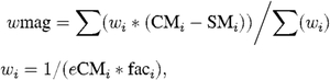
where the weights are the inverse of the catalog errors (eCM) in magnitudes, scaled by factors determined empirically to optimize the fits. After experimentation with data sets where cross-checks are available, we chose factors of {6,4,3,4,4} for UBVRI, {6,4,2,3,3} for u′ g′ r′ i′ z′, and {1,1,1.5,1,1.3,1.3} for BT VT RN J2 H2 K2/S. All the filter bands display broad, shallow minima of synthetic catalog error with factor, and there is some cross talk between bands. The results are not critically dependent on these factors: they are much more dependent on the catalog photometric errors themselves. But the factors were selected within these broad minima to minimize the rms errors in each band and to improve the consistency of spectral type fitting between different fits.
Smaller factors imply higher weights, although the weighting also depends on the catalog magnitude errors, so the weighting for NOMAD RN (dispersion 0.25 mag, factor 1.5) is usually least. Larger factors are necessary for data with small intrinsic errors, because the library spectra cannot achieve millimagnitude fits to the data. The factors are not completely independent, but are interconnected by the library spectra themselves. Fitted magnitudes in U/u′ or B/g′, for instance, can be improved slightly by reducing the scale factor for these bands, but at the expense of slightly worse fits in redder bands. This tends to indicate spectral library calibration errors in the U/u′ region.
For each filter band to be fitted, we then form

and form a χ2 normalized by the number of filters:

The resultant χ2 will be dominated by those bands where dMi exceeds eCMi.
Additionally, we can form rms magnitude error values for the six Tycho2/NOMAD RN/2MASS, five Landolt, five Sloan, and three 2MASS bands when they are available, as
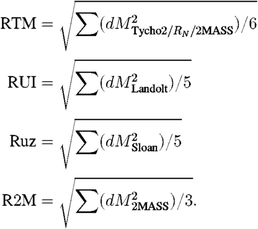
The rms values without the influence of U/u′ can also be formed: e.g., RBI and Rgz.
The spectral matching process also computes a distance modulus using the adopted absolute V magnitude from Table 6 and the fitted (apparent) V magnitude (and hence a distance estimate in parsecs for each fit):

For each program star we get an ordered list of 141 values of χ2, one for each spectrum, where the optimum spectrum has the lowest χ2. Good fits normally have χ2 ≤ 1 because of the normalization by photometric errors and number of filters, but higher values are possible when there are significant differences between catalog and synthetic magnitudes in one or more bands
Several fits at the top of the ordered list may have close, and good, fits. These typically represent uncertainty between close spectral types; metal-rich spectra of slightly earlier types; metal-weak spectra of later types; or confusion between dwarf, giant, or even supergiant spectra of similar colors.
Additional constraints used to discriminate between these cases are described subsequently. The predicted magnitudes of fits with similar χ2 values are themselves similar to within 1–3%. The predicted distances can vary widely, however, particularly when there are close dwarf and giant matches.
5.2. Distance Constraints
We can use the (J - H, H - K) color-color diagram as in Bessell & Brett (1988; Fig. 5) to discriminate between late-type dwarfs and giants. We have adopted the simple criterion that an M star fitted type must be a dwarf if the 2MASS colors (H2 - K2) > 0.23 and (J2 - H2) < 0.75.
Luminosity class discrimination can also be based on any available distance information, including proper motions listed in the Tycho2 catalog. The Hipparcos catalog displays a fairly good relation between parallax and proper motion (PM):

where  Expressed as a limit, where we adopt the outer boundary of the relation, this is

The proper motions listed in the Tycho2 catalog can therefore be used, with some caution, to check derived distances. Small measured proper motions do not provide a significant limit to distance, but large measured proper motions can be used to discriminate between giant fits at many kiloparsecs or nearer subgiants or dwarfs. We did not use parallax measurements directly to determine distance, as they are not available for most catalog stars.
For catalog stars with low or no known proper motion, we set a somewhat arbitrary Galactic upper distance limit of 20 kpc. This usually excludes supergiants, except where the catalog star is bright, but does not exclude giant fits. We do not make any allowance for reddening in our spectral fits or in our distance estimates.
We also adopt a lower distance limit of 3 pc, which excludes some very nearby dwarf fits (e.g., at a distance of 0 pc) in favor of brighter candidates. There are several nearby stars in the Tycho2 catalog, however, including Barnard’s star (BD + 04 3561a fitted as an M3V at a distance of 5 pc; an M4.2V fit at 2.9 pc was excluded by our lower distance limit), Lalande21185 (BD + 36 2147 fitted as an M1.9V at 4 pc), Ross154 (fitted as an M4.2V at 5 pc), Epsilon Eridani (BD-09 697 fitted erroneously as a G5 III at 12 pc; a K2V fit at 3 pc occurs at a lower rank), Groombridge 34 (GJ15 fitted as an M1.9V at 5 pc), Epsilon Indi (CPD-57 10015 fitted as a K4V at 3 pc), Luyten’s star (BD + 05 1668 fitted as an M3V at 6 pc), Kapteyn’s star (CD-45 1841 fitted as an M2.5V at 7 pc), Wolf 1061 (fitted as an M4.2 at 4 pc), Gliese 1 (fitted as an M1.9V at 6 pc), GJ687 (BD + 68 946 fitted as an M3V at 5 pc), GJ674 (fitted as an M3V at 5 pc), GJ440 (WD1142-645 fitted as an L749-DBQ4 type WD at 5 pc), Groombridge 1618 (GJ380 fitted as an M1V at 3 pc), and AD Leonis (fitted as an M3V at 5 pc).
We always accept the highest-ranked spectrum (lowest χ2) unless we have proper motion, distance limit, or color information to exclude a top-ranked giant or supergiant fit.
In the case that the top-ranked spectral fit contravenes one of the preceding four criteria, our process descends the list of rank-ordered χ2 fits to the first fit that is compliant with our distance constraints. This additional test increases the χ2 value, but often not by very much. In checks of Tycho2/NOMAD/2MASS (TNM) fits where we also have Sloan or Landolt information, it increases the RTM values, but can reduce the RUI or Ruz values.
Our checks indicate that the (relatively noisy) TNM fits can select giant fits over dwarf fits more often than do fits with better optical data. Nevertheless, for TNM fits we have set our proper-motion/distance limit very conservatively, modifying the selected fit only when the predicted distance is clearly too large. There is therefore some residual bias in the TNM fits toward giants over dwarfs. The rank of each accepted fit is listed in the results, and the predicted distances can be checked against the Tycho2 proper motions.
We have used SM29 and Enthought Python30 for most of the data processing; these scripts are available on request. By judicious use of NumPy arrays we can fit ∼1 million stars in eight bands with 141 sets of library magnitudes in about 10 minutes on a typical single CPU, so processing time is not a limiting factor.
5.3. Accuracy of the Spectral Matching Process
The library spectra typically have relatively high signal-to-noise ratio, but are limited by their own flux calibration uncertainties, particularly in the U band, which, unlike the uv, was observed from the ground. In approximate order of decreasing uncertainty, the accuracy of our spectrally fitted magnitudes is limited by the following accuracies:
- 1.The input catalog magnitudes
- 2.The spectral matching process, discussed subsequently
- 3.The adopted system transmission functions, discussed in § 3
- 4.
- 5.Our library spectra, particularly in U
- 6.The CALSPEC spectra
The first item is usually largest, but it is noteworthy that our fits to catalog values, where they can be properly checked, approach (and sometimes exceed) the accuracy of the catalogs themselves.
The methodology presented here cannot (yet) approach the goal of less than1% photometry and is fundamentally limited by the accuracy of the CALSPEC spectra, currently to about 2%. In some ways, it avoids the end-to-end calibration of telescopes and detectors (discussed, for instance, in Stubbs & Tonry 2006), but complements it by offering an easy way to monitor total system throughput by enabling automatic pipelined measurements for wider-field images.
The issues of atmospheric variability in nominally photometric conditions are discussed in Sung & Bessell (2000) and McGraw et al. (2010). The methodology presented here is currently less accurate than the expected atmospheric changes for field-to-field comparisons. But using standards in each digital field, rather than transferring them, offers the advantage of both monitoring and consistently removing such variability within the same field, even during known nonphotometric conditions.
6. PRIMARY STANDARDS
6.1. Landolt Standards with 2MASS
We illustrate the spectral matching process by matching library spectra to 594 Landolt standards with accurate UBVRI magnitudes, for which we also have 2MASS JHK2/S magnitudes.
We took the updated Landolt coordinates, magnitudes, uncertainties, and proper motions from Landolt (2009). We used the find2mass tool in the cdsclient package from Centers de Données (CDS)31 to check 2MASS matches within 3" to these coordinates and found good correspondence to Landolt (2009) for all except SA92-260 and SA109-956. For these last two stars we have adjusted the coordinates and matching 2MASS magnitudes, checking them with Landolt finding charts and DSS images. As indicated in Landolt (2009) the star E near the T-Phe variable star has a NOMAD entry but no 2MASS entry within 30"; it has been excluded from our list here.
For each standard, we compute the χ2 value for each of 141 library spectral magnitudes, as described in § 5 for the eight L2M bands: Landolt UBVRI and 2MASS JHK2/S. We then order them by χ2, check against our distance constraints, and select the one that satisfies the constraints with the best match to the eight catalog magnitudes.
The results are listed in Table 7, which lists the standard name; coordinates; Landolt magnitudes and colors; number of observations; spectral type from Drilling & Landolt (1979); fitted rank; χ2 values; two rms errors in Landolt magnitudes RUI and RBI; fitted spectral library number and type; fitted magnitudes in BT VT, JHK2/S, UBVRI, UKIRT ZV YV, and Sloan u′ g′ r′ i′ z′; and distance in parsecs. Magnitude values in other bandpasses can be derived by adding the library magnitude from Table 6 for the appropriate band and spectral type to the fitted V magnitude.
There is reasonably good correspondence between the objective prism spectral types from Drilling & Landolt (1979) and those fitted here—about 123 close matches versus 13 discrepant types—with the worst two being SA110-499 and SA110-450.
The catalog data for the Landolt standards—sexagesimal coordinates; UBVRI magnitudes and errors; 2MASS magnitudes, errors, and coordinates in degrees; and UKIRT ZY and JHKMKO data, where available—are listed in Table 8. When Landolt (2009) photometric errors were left blank, indicating one or few standard observations, we have set them to 0.009 mag for the purpose of our fitting process.
Figure 10 shows the eight-band L2M fitted magnitudes plotted as Fit–Landolt magnitudes against their Landolt standard values for BVRI. The display range excludes a few outliers discussed subsequently. The dashed-line histograms of number (to the right) vs. delta magnitude (ordinate) illustrate that most stars lie close to the zero-delta line. The clipped 1σ dispersions are 0.05, 0.03, 0.04, and 0.05 mag for BVRI, respectively. In order to compute these dispersions we formed a sigma for each of BVRI separately, performed a 3σ clip, then repeated a second (tighter) 3σ clip to arrive at the quoted 1σ dispersions. This typically clips 4–8% of the values, or 25–45 of the values here, but retains about 95% of the values.
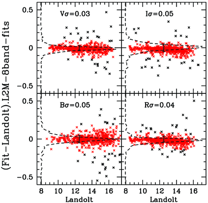
Fig. 10.— BVRI fits with eight L2M UBVRI - JHK2/S bands for 594 Landolt standards. The data are plotted as magnitude differences Fit-Landolt on the ordinate vs. Landolt catalog magnitudes on the abscissa. Black crosses indicate points excluded by sigma clipping; the scaling excludes a few outliers discussed in the text.Red points indicate those remaining after sigma clipping. The dashed-line histograms plotted vertically in each panel illustrate the number distribution of all the points about the zero-delta (horizontal) line. Clipped ± 1σ errors are indicated in each panel caption and by the vertical error bars.
Of the clipped values, almost two-thirds have been observed only once or twice in Table 8; the others are mainly white dwarfs, very red stars, or perhaps double stars. A few poor fits with large values of χ2 and RUI include some late giants and supergiants when the spectral library coverage is weak and Feige24, a double star, which is fairly well fit with a double-star spectrum constructed from a 68∶32% mix at a V band of DA1 (GD71) and K4V spectra. PG1530 + 057 is listed as a uv -emission source and is also best fit with this DA/K4 dwarf double-star spectrum, as is SA107-215. No effort was made to optimize these coincidental double-spectrum fits, but they emphasize that double stars are likely to be present among Landolt standards, as among other catalog stars.
In many cases of multiple stars within the observing aperture, including known doubles like BD + 26 2606, the spectral flux will be sufficiently dominated by one spectrum at all wavelengths that fitting to a single spectral type is valid. But some data do show the predominant influence of one spectrum in the blue and another in the red. Most stars here (∼94%, or 560) are very well fit by the (single) spectral matching process.
The clipped 1σ dispersion for U shown in Figure 11 is 0.16 mag; 0.12 mag to U < 16 and increasing for fainter magnitudes. The four faintest U standards were not observed often in Landolt (2009). Our fits for these find brighter U values, but have fairly large χ2 and RUI.
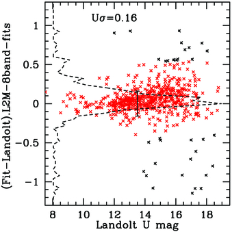
Fig. 11.— U -band fits with eight L2M UBVRI - JHK2/S bands plotted as Fit-Landolt for 594 Landolt standards.Red crosses indicate points retained after sigma clipping, and the dashed-line histogram illustrates the number distribution of all the points around the zero-delta line. The sigma is 0.12 mag to U < 16, increasing for fainter stars.
The distribution of spectrally fitted types and luminosities for Landolt standards is shown graphically as an HR diagram in Figure 12. The fitted types are plotted as absolute V magnitudes vs. V - I color, with different symbols for different luminosity classes and metallicities. The area of each symbol is proportional to the number of fitted stars of that type. The truncation of the lower main sequence is, of course, a brightness selection effect. The Landolt primary standards cover a wide range of colors, types, and metallicities, with most MK types well represented.
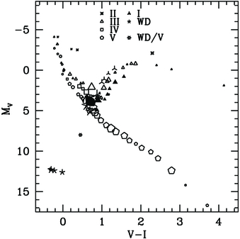
Fig. 12.— HR diagram for 594 Landolt standards shows our fitted types as absolute V magnitudes vs. spectral library V - I colors. Dwarfs are represented as pentagons, subgiants are squares, giants are triangles, and luminosity classes II and I are four-point and three-point stars, respectively. White dwarfs are shown as five-point crosses. Metal-weak dwarfs and giants are shown as five- or three-sided crosses, and metal-rich components are five- or three-sided filled symbols. The area of each symbol is proportional to the number of stars fitted with that library spectrum. The six-starred symbol at (0.45,8) represents the DA1/K4V double spectral type, fitted to Feige24, PG1530 + 057A, and SA107-215.
6.1.1. ZY on Vega and AB Systems
Table 8 also contains ZV YV data from UKIRT for 14 standards and JHKMKO for 17 Landolt standards (see § 1). The 1σ dispersions (not shown) for both ZV and YV are 0.06 mag for 14 stars with standard values (including two CALSPEC standards: GD 50 fit with a GD 153 DA0 type spectrum and GD 71 fit with its own library GD 71 DA1 spectrum).
Despite the fact that the ZV bandpass terminates shortward of z or z′, and because of the falling long-wavelength response of CCDs, the pivot wavelengths of ZV and z′ in Table 3 are similar. It is therefore not surprising that there is a simple one-to-one relation between fitted values for ZV on the Vega system and z′ and z on the AB system, which holds for 14 Landolt/Sloan standards and also for 594 fitted values for Landolt standards and for the spectral library magnitude data in Table 6, both of which cover a wide color range:

where the additive constant is simply the derived zero point for ZV (and that for zAB is zero). This is equivalent to the magnitude difference between the Vega and AB system zero-magnitude fluxes at ZV: 0.58 = -2.5 ∗ log 10(2128/3631) from Table 3.
For AB magnitudes measured with a bandpass similar to YV used by UKIRT/WFCAM, the relation between the YV Vega and AB system magnitudes should also be the Vega to AB zero-point offset at this bandpass: i.e.,

where KY should be close to 0.61 - 0.0 or, alternatively, to the difference in magnitudes between the 0 mag flux at YV on the Vega system and 0 mag (3631 Jy) for the AB system: i.e., 0.61 = -2.5 ∗ log 10(2072/3631) from Table 3.
Care must be taken, however, particularly with Y -band measurements made with CCDs, because CCD QEs fall very fast in the 1.0–1.1 μ region, and CCD Y -bandpass profiles are necessarily quite different from the rectangular UKIRT WFCAM HgCdTe YV bandpass (see Fig. 2). Many CCDs have little or no sensitivity at the Y band. Deep-depletion CCDs can have significant QE out to the silicon bandgap at 1.1 μ, but CCDs even of the same type may have varying QE curves and system bandpasses at Y and hence also have different effective and pivot wavelengths.
At LCOGT we use the Pan-STARRS type of ZS (for Z -short) and Y filters with our Merope E2V 42-40 CCDs on Faulkes Telescopes North and South (FTN and FTS). Our LCOGT ZS YE system bandpasses (including filter, atmosphere, and detector) are illustrated in Figure 2. We refer to YE to specifically reference the Pan-STARRS type of Y bandpass with our E2V system QE curve and 1.3 air masses of extinction at a typical elevation of 2100 m. The measured pivot wavelengths for ZV and ZS are 877.6 and 865.1 nm, respectively; those for YV and YE are 1020.8 and 989.9 nm, respectively. The effective wavelengths for either type of Z and Y bandpasses vary by less than 1% and 0.5%, respectively, however, from white dwarf to M dwarf spectra, so Z/Y -band measurements can provide convenient near-infrared flux and temperature measurements, enabling quite good dwarf/giant discrimination for M stars, somewhat insulated from atmospheric and stellar spectral features.
For the same (few) standards shown in Table 3 we obtain zero points (on the Vega system): ZS = 0.56 ± 0.04 and YE = 0.55 ± 0.03. We can form ZS YE filter system magnitudes for all the spectral library stars and form linear relationships with ZV YV of the same stars, but because of the bandpass differences they are no longer simply one-to-one relationships of unit slope. For synthetic measurements with LCOGT ZS YE of our 141 spectral library standards in Table 6 we obtain

where ZS YE and YV are on the Vega system. These relations are dependent on the particular bandpasses used here, but indicate that CCD-based Y -band magnitudes (on either the Vega or AB systems) can be successfully tied to the UKIRT/WFCAM Y -band standard system, with CCD-system-dependent equations.
6.1.2. JHKMKO Fits
Our fitted values of JHKMKO on the Vega system match 17 Landolt stars with standard UKIRT values,32 which further supports our derivation of their zero points:
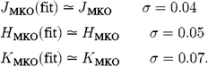
J - H and H - K fitted colors form linear relationships with J - HMKO and H - KMKO for these same 17 stars with sigmas of 0.04 and 0.03 mag, respectively, but with little color range. There are color terms between the JHKMKO and 2MASS JHK2/S systems.
6.2. Sloan Standards
There are 158 Sloan standards listed in Table 9, together with UKIRT values of ZV YV and JHKMKO where available, and 2MASS values of JHK2/S. These have been spectrally matched with eight S2M bands of u′ g′ r′ i′ z′ J2 H2 K2, and their fitted values of Landolt and Sloan magnitudes and distances in parsecs are listed in Table 10. The comparisons with standard data are discussed subsequently.
6.3. Landolt/Sloan/Tycho2/2MASS Standards
There are 96 standards in common between the Landolt and Sloan lists; they all have 2MASS J2 H2 K2/S and NOMAD RN magnitudes; 65 of these also have Tycho2 BT VT magnitudes. This very small sample with cross-referenced data provides useful illustrations of the strengths and limitations of the spectral matching process.
Table 11 lists Landolt, Sloan, NOMAD, 2MASS, and Tycho2 magnitudes, errors, coordinates, and proper motions. In this case the proper motions are from Tycho2; they are similar to but slightly different from proper motions listed in Table 8, which are from Landolt (2009). The proper motions are only used to discriminate distance limits here.
These stellar magnitudes have been fitted four ways:
- 1.They were fitted with UBVRI, u′ g′ r′ i′ z′, and BT VT J2 H2 K2/S, for a total of 15 bands.
- 2.They were fitted with Landolt and 2MASS data (L2M), for a total of eight bands.
- 3.They were fitted with Sloan and 2MASS data (S2M), for a total of eight bands
- 4.They were fitted with Tycho2, NOMAD RN, and 2MASS data (TNM), for a total of six bands.
The fits are listed in Table 12, where the results are listed in full for the first method, then only for those stars with different matching spectra for subsequent fits.
In each case the fitting process produces synthesized magnitudes at all bands, together with library types and distances. The synthesized magnitudes were compared with the standard values, and the fitted library types were checked for consistency between fits.
6.3.1. Examples of Spectral Matching
Figure 13 shows the S2M eight-band fit for SA93-424, a K1 III at 768 pc, with F(ν) plotted against wavelength. The same K1 III fit is obtained with the 15-band fit and the L2M eight-band fit; i.e., the fits have the same type and the scale is different by less than 0.2%. For this fit, RUI, Ruz, and RTM rms values are 0.02, 0.03, and 0.16 mag, respectively. Overplotted (blackdashed line) is the best-fit rK0 III type at 393 pc obtained with the TNM fit (six bands). The six-band fit is forced a bit brighter in the optical region by the BT VT data, but matches the K2/S point better. The latter fit gives synthesized Landolt-Sloan magnitudes with RUI, Ruz, and RTM of 0.16, 0.09, and 0.18 mag, respectively. Drilling & Landolt (1979) list a G8 III spectral type for SA93-424, from objective prism spectra.
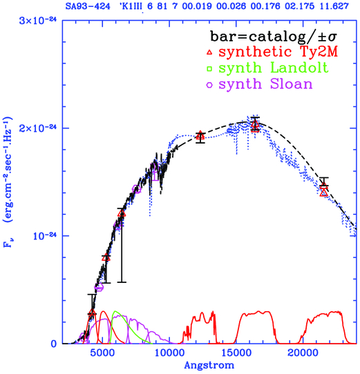
Fig. 13.— S2M eight-band K1 III fit for SA93-424 is shown (fainter,blue dotted trace) as F(ν) vs. wavelength. The Sloan filter profiles are shown in magenta, the Tycho2/2MASS profiles are shown in red and the R profile (matched here to NOMAD RN are shown in green. Bars (black, green, and magenta) identify the Tycho2/2MASS, Landolt (and RN), and Sloan catalog magnitudes and errors. Triangles (red), squares (green), and circles (magenta) identify fitted synthetic fluxes and magnitudes in the same systems. The overlaid black dashed-line spectrum is the rK0 III fit obtained with six TNM bands. The long vertical black bar represents the RN catalog error, scaled by a factor 1.5, on the second fit. The catalog fluxes are at the center of each bar, and the synthesized fluxes are marked by the symbols.
Figure 14 shows the L2M fit for BD + 02 2711, a B3 III at 5.2 kpc, plotted as a blue dotted line, with RUI, Ruz, and RTM values of 0.04, 0.05, and 0.08 mag. The S2M and 15-band fits are similar. The six-band TNM fit of a GRW + 70 5824 (DA3) type white dwarf at 4 pc is shown as the overplotted black dashed line, with RUI, Ruz, and RTM values of 0.13, 0.14, and 0.07 mag, respectively. The latter fit is a better match to the Tycho2 bands, but is unconstrained at wavelengths shorter than BT and is a poorer fit to the Landolt and Sloan bands. There is no objective prism type for BD + 02 2711 from Drilling & Landolt (1979), but SIMBAD lists a type of B5V at a distance (from its Hipparcos parallax) of 1.3 kpc. An early B dwarf type was selected as a high, but not top-ranked, fit by all the spectral matches.
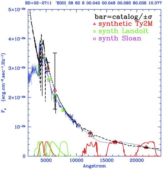
Fig. 14.— L2M eight-band B3 III fit is shown (lower,blue dotted line) as F(ν) vs. wavelength. The six Tycho 2/RN/2MASS (six-band, TNM) DA3-WD fit is shown as the overlaid black dashed-line trace. The long vertical black bar represents the NOMAD RN magnitude (in its center) and error for the TNM fit, with a red triangle for the synthesized flux. The green bar (above the fitted green square) represents the Landolt R catalog magnitude and error for this star. Symbols are as in Fig. 12.
These examples were chosen to illustrate both the successes and limitations of the spectral matching method. They emphasize that color or spectral type are matched better than luminosity class, particularly when the input photometric errors are larger, but that good magnitude fits can be obtained in most cases.
Figure 15 shows the first-ranked S2M fit for SA102-620: a K4V at 38 pc. The K4V fit is also obtained as the second-ranked fits with the 15-band and the eight-band L2M fits, where a slightly higher ranked K2 III fit at 540 pc was rejected in these two cases as being beyond a calculated proper-motion-limited distance of 285 pc. For the S2M fit, RUI, Ruz, and RTM values are 0.06, 0.08, and 0.05 mag, respectively. Overplotted (blackdashed line) is the second-ranked six-band TNM fit rK1 III at 200 pc, which is a bit bluer in the optical region because of the BT VT RN data. The latter fit has RUI, Ruz, and RTM values of 0.11, 0.13, and 0.06 mag, respectively; Drilling & Landolt (1979) list an M0 III type for SA102-620. SIMBAD lists a K5 III type, but with a parallax (from Hipparcos) of 22 mas, implying a distance of 45 pc; i.e., the star must be a dwarf. The K4V L2M and S2M fits are best, but the TNM rK1 III fit still matches the magnitudes quite well.
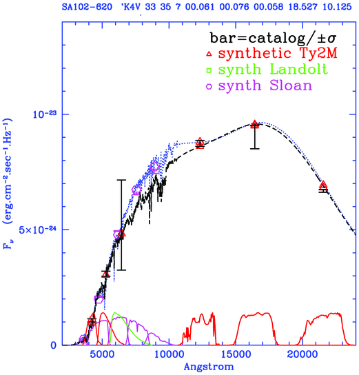
Fig. 15.— S2M eight-band K4 V fit for SA102-620 is shown (bluedotted line) as F(ν) vs. wavelength. The overlaid black dashed-line spectrum is the rK1 III fit obtained with 6 Tycho 2/RN/2MASS bands. Symbols are as in Fig. 12.
Figure 16 compares three types of fit for the Table 11 sample. The fitted BVRI magnitudes are plotted as Fit–Landolt on the ordinate vs. Landolt catalog values on the abscissa. A plot of Fit-Sloan vs. Sloan catalog magnitudes shows similar dispersions. The clipped sigmas, typically containing more than 92% of the points, are 0.12, 0.03, 0.02, 0.03, and 0.03 mag and 0.13, 0.03, 0.03, 0.03, and 0.04 mag for UBVRI and u′ g′ r′ i′ z′ bands, respectively, for the eight-band L2M fits. They are 0.14, 0.06, 0.03, 0.02, and 0.03 mag and 0.15, 0.03, 0.02, 0.02, and 0.03 mag for UBVRI and u′ g′ r′ i′ z′ bands, respectively, for the eight-band S2M fits, and they are 0.21, 0.15, 0.12, 0.10, and 0.08 mag and 0.19, 0.15, 0.11, 0.09, and 0.07 mag for UBVRI and u′ g′ r′ i′ z′ bands, respectively, for the six-band TNM fits. The latter TNM sigmas, combined and averaged for UBVRI and u′ g′ r′ i′ z′ as ∼0.2, 0.15, 0.12, 0.10, and 0.08 mag, are reported as the typical 1σ error per Tycho2 star per band in the Abstract and can be compared with the TNM g′ r′ i′ z′ fits reported in § 7.
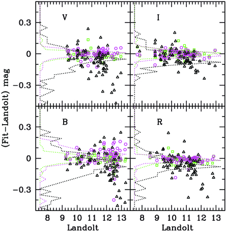
Fig. 16.— Landolt BVRI fits for 65 stars with Landolt, Sloan, Tycho2, NOMAD, and 2MASS standard magnitudes. The fitted BVRI magnitudes on the ordinate are plotted as Fit-Landolt vs. the catalog values on the abscissa. U fits are not shown. Squares (green) and histogram indicate the L2M fits obtained with five Landolt and three 2MASS magnitudes, magenta circles and histogram indicate the S2M fits obtained with five Sloan and three 2MASS magnitudes, and black triangles and the wider histogram indicate the TNM fits obtained with BT VT RN and three 2MASS magnitudes. The green and magenta L2M and S2M histograms are narrow, indicating good fits to the zero-delta line. The black TNM histogram is wider, as expected for these TNM fits.
6.3.2. Accuracy and Consistency of the Fits
It can be seen that there is good correspondence between the UBVRI and u′ g′ r′ i′ z′ bandpass sigmas when we are able to compare them directly. This is natural, because the fits depend primarily on the catalog errors and the spectral library errors, not on any mismatch between Landolt and Sloan systems (see § 5.3). In other cases we are only able to measure the quality of fit in either Landolt or Sloan bands, but we can infer that the quality of fit for the other system will be quantitatively similar.
Landolt UBVRI magnitudes can also be derived in this simple case with accurate Sloan u′ g′ r′ i′ z′ magnitudes, using the formulas from Jester et al. (2005). For these 65 stars this results in sigmas of 0.06, 0.05, 0.03, 0.04, and 0.04 for UBVRI, respectively. The spectral matching method for L2M and S2M methods are therefore comparable with, or better than, the Jester et al. (2005) method for BVRI and griz bands, but worse for U/u. The TNM fits are less accurate, but generally fit better at BVR bands, than the BT VT RN errors themselves. They therefore offer a reliable fitting method in the absence of more accurate optical data.
Note that the Jester formulas are susceptible to errors in just one filter that can propagate to several fitted filter bands. The spectral matching process is not immune to input catalog errors but, by giving lower weight to discrepant points with larger photometric errors, can provide more robust synthetic fits in all bands.
The fitted spectral types can vary according to the input data matched, but the results are generally consistent. Figure 17 illustrates our derived distributions of stellar types and luminosities for 65 Landolt/Sloan standards, binned into 141 library spectral types and plotted as adopted absolute V magnitudes against their V - I colors. The same symbols for different luminosity classes and different metallicities are used from Figure 12, and the symbol area is proportional to the number of stars in each library type bin.
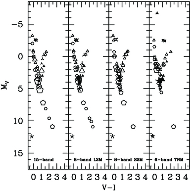
Fig. 17.— HR diagram for 65 Landolt/Sloan standards shows our fitted types as adopted absolute V magnitudes vs. spectral library V - I colors, for four different fits. Symbols are as in Fig. 12. The area of each symbol is proportional to the number of stars fitted with that library spectrum.
The first fit on the left is for all 15 Landolt, Sloan, and Tycho2/2MASS bands. The second fit is for the eight-band L2M fits, the third is for the eight-band S2M fits, and the fourth is on the right for the six-band TNM fits.
These fits and their distributions of selected spectral types and luminosities are different in detail, but similar statistically, and produce closely similar magnitude fits.
The HR diagram on the right illustrates that TNM fits show a slight preference for giant, rather than dwarf, types. The TNM fits also select one supergiant for SA97-351, an F0I at a distance of 19 kpc (just inside our distance limit), rather than an A7V at 342 pc (L2M) or F0 III at 553 pc (S2M). Drilling & Landolt (1979) list an objective prism spectral type of A0 for SA97-351.
There are 27 matches and 19 close matches between the L2M and S2M fits. There are 14 matches and 21 close matches between the S2M and TNM fits. In all cases the fitted spectra and derived magnitudes are similar, as shown in Figure 16.
The difference in optimal fits, depending on the number and accuracy of filter photometry available, illustrates both the strengths and limitations of the spectral matching process and of the spectral library. The library quantization is too fine for this purpose in some places and insufficiently sampled in others. In general, the spectral matching process is better at determining the spectral type than the luminosity class.
The differences between accurate and lower-quality photometric data are apparent. Nevertheless, the spectral matching process works well even for poorly determined optical photometry, where the more accurate 2MASS data help constrain the fitted spectra in both type and magnitude scale.
Better spectral type discrimination is possible when more accurate filter data are available, but the fitted magnitudes are similar in all these cases, within the quoted errors. Fitted spectral types are more accurate than luminosity class. The fitted distance estimates can be used as a sanity check on the derived fit.
7. SECONDARY SDSS STANDARDS
7.1. SDSS-PT Observations
Tucker et al. (2006) and Davenport et al. (2007) have published lists of almost 3.2 million SDSS observations in g′ r′ i′ z′.33 These were observed on the US Naval Observatory PT and used to calibrate the SDSS survey scans.34 They are more accurate than survey data, as evidenced by the consistency of their repeated observations and (small) errors. We use them here as secondary standard calibrators. We first combined the lists to produce a list of ∼1 million repeated observations, with photometric errors being the maximum of any single observation, or the rms of the average if that was greater. These were matched against 2MASS stars within 3" to produce a slightly shorter list of stars that reach as faint as g′ ∼ 21 mag and are discussed in § 8.2.
This list was further matched against the Tycho2 and NOMAD catalogs to produce a smaller list of 10,926 SDSS-PT standards with BT VT RN and reaching as faint as g′ ≃ 13.5 mag. These were fitted two ways: (1) S2M with seven bands (g′ r′ i′ z′ and JHK2/S) and (2) TNM with six bands (BT VT RN J2 H2 K2/S), and their results were compared with the PT standard values.
Figure 18 shows the S2M g′ r′ i′ z′ fits to the ∼11,000 SDSS-PT/2MASS stars with Tycho2/NOMAD data, with sigmas of 0.03, 0.02, 0.02, and 0.03 in g′ r′ i′ z′, respectively, after clipping outliers, but retaining more than 96% of the points in each band. The sigma in g′ is 0.07 mag for ∼11,000 stars, but the red dots show a sigma of 0.03 mag after clipping about 400 outliers. This illustrates typical 1σ errors for accurate SDSS data coupled with 2MASS data. The histograms illustrate the number distributions of errors about the mean for all the points where they become overlapped and blurred.
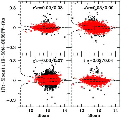
Fig. 18.— S2M fits with seven g′ r′ i′ z′ - JHK2/S bands for ∼11,000 SDSS-PT standards with 2MASS, NOMAD, and Tycho2 photometry, plotted as (Fit-Sloan) vs. Sloan magnitudes. Black crosses are points rejected by the sigma clipping, and red points are those remaining after sigma clipping. The clipped points overlap, but the number distributions for all the points about the zero-delta line are indicated by the dashed-line histograms. The sigmas indicated in the panel captions are for the clipped/and all the stars in each band, with ± 1σ error bars drawn for the former.
From § 6.3.2 we infer that the errors for BVRI are similar. The sigmas for fitted JHK2/S are 0.04, 0.04, 0.03 mag, respectively.
Figure 19 shows the corresponding TNM fits to these stars, with clipped and unclipped sigmas of 0.15/0.25, 0.12/0.16, 0.09/0.13, and 0.07/0.15 mag in g′ r′ i′ z′, respectively, after clipping outliers (shown in black) but leaving 78% of the red points in g′ and more than 88% of the red points in the other three colors. We again infer that these illustrate typical 1σ errors for both griz and BVRI fits to the Tycho2 catalog when coupled with NOMAD and 2MASS magnitudes and note their similarity to typical TNM errors quoted in § 6.3.1 and the Abstract. The histograms show the number distribution of errors about the mean for all the TNM fits to ∼11,000 SDSS-PT/2MASS/Tycho2 stars.
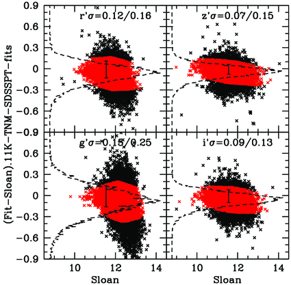
Fig. 19.— TNM fits with six BT VT RN - JHK2/S bands for the same ∼11,000 SDSS-PT standards plotted as Fit-Sloan vs. Sloan magnitudes. Note the vertical scale change from the previous figure. Black crosses show all the stars. The red points in the middle show 80–90% of stars remaining after sigma clipping. Sigmas after and before clipping are indicated. The histograms show the number distribution of errors about the mean for all the points. There may be some bias toward brighter fitted magnitudes in at least the g′ r′ bands, but the errors are dominated here by the input Tycho2/NOMAD catalog accuracies.
The TNM fit errors quoted here for r′ i′ z′ are similar to those found by Ofek (2008), but for a larger magnitude range. The error quoted for g′ band is slightly larger than previously reported, but for a wider fitted magnitude range. The sigmas for fitted JHK2/S are 0.03, 0.02, and 0.02 mag, respectively.
7.2. Southern SDSS Standards
Smith et al. (2005) have published a list of ∼16,000 southern SDSS standards,35 which includes some repetition. We matched 15,673 of these to 2MASS catalog values and fitted them in eight S2M bands: u′ g′ r′ i′ z′ and JHK2/S. The clipped and unclipped 1σ fits are 0.22/0.51, 0.08/0.22, 0.04/0.07, 0.07/0.16, and 0.11/0.25 mag for u′ g′ r′ i′ z′, respectively, for all Sloan southern stars ranging up to g ∼ 19 mag, as shown in Figure 20. The vertical histograms show the number distribution of errors about the mean for all these southern Sloan stars and indicate that our fits produce an excess of rejected fits fainter than the catalog values in z′ and, to a lesser extent, in i′.
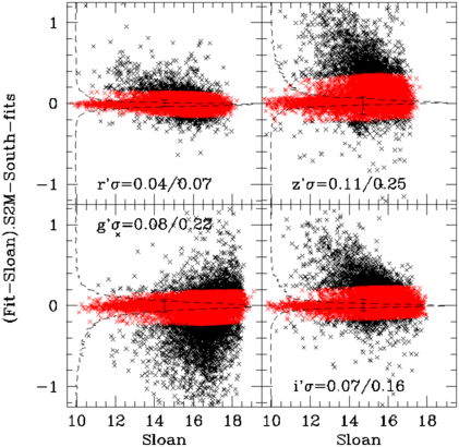
Fig. 20.— S2M fits with eight ugriz - JHK2/S bands for ∼16,000 southern SDSS standards, to g′ ∼ 19 mag. Clipped/unclipped sigmas, histograms, and error bars as before.
The JHK2 fits are not shown, but the J2 fit shows a corresponding excess of fitted points brighter than the catalog values, whereas the HK2 fits are symmetrically distributed about the mean-delta (zero) line. Thus, our fits to southern Sloan i′ z′ are being pushed slightly fainter at the red end by the usually reliable 2MASS data.
There are ∼6000 stars with g′ < 16 : for these stars the clipped sigmas are 0.13, 0.07, 0.04, 0.06, and 0.09 in u′ g′ r′ i′ z′, respectively: i.e., not as good as for the SDSS-PT stars in Figure 18, but for a larger magnitude range in this case.
The HR diagram for this fit is shown in Figure 21. Compared with the Landolt distribution in Figure 12, this shows a slightly less populated lower main sequence, more stars near the main sequence turnoff, a slightly better defined red giant branch out to M8 III, and some horizontal branch type giants but no supergiants.
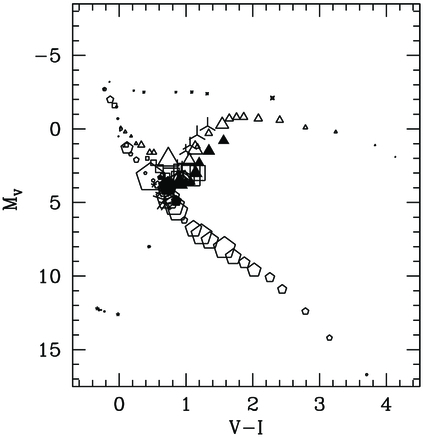
Fig. 21.— HR diagram for ∼16,000 SDSS southern standards. Symbols are as in Fig. 12.
We have further matched this list to Tycho2 BT VT and NOMAD RN magnitudes, resulting in a list of only 201 southern stars, as most of the southern SDSS standards are too faint to have Tycho2 matches. The comparison of fitted griz magnitudes to standard values for fits using six TNM bands is shown in Figure 22, with sigmas of 0.23, 0.16, 0.12, 0.11, and 0.09 mag in ugriz, respectively, and comparable with the TNM fits to the preceding SDSS-PT stars for a similar magnitude range.
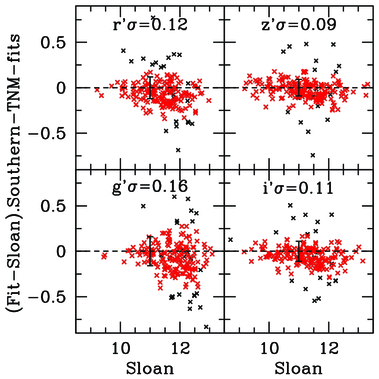
Fig. 22.— TNM fits with six BT VT RN - JHK2/S bands for 201 southern SDSS standards with NOMAD and Tycho2 magnitudes. The fits for g′ r′ i′ z′ are plotted as Fit-Sloan vs. Sloan magnitudes, with the clipped data shown as red crosses, with their clipped sigmas indicated in the panels, and as error bars. The black crosses were rejected by the sigma clipping process.
8. CATALOGS
8.1. Landolt and Sloan Fitted Data
Landolt standards—including updated coordinates, magnitudes, and errors; JHK2/S 2MASS data; and UKIRT ZV YV JHKMKO data, where known—are listed for 594 stars in Table 8. Table 7 contains the spectrally fitted rank, χ2, RUI, RBI, library number and type, fitted magnitudes BT VT J2 H2 K2 UBVRIZV YV, u′ g′ r′ i′ z, and distances in parsecs.
Similar data are contained in Tables 9 and 10 for Sloan standards and in Tables 11 and 12 for stars common to both lists, as described in § 6.
8.2. Secondary Standard Fitted Data
Table 13 contains coordinates, standard magnitudes, and errors in g′ r′ i′ z′; number of repeated PT observations; merged J2 H2 K2 2MASS data; fitted Rgz, R2M (2MASS), library types, UBVRI - ZV YV, and u′ g′ r′ i′ z′ magnitudes and distances for ∼1 million SDSS-PT stars.
Figure 23 shows the seven-band S2M fits for these stars. The outer black dots show all the rejected stars, and the red narrower bands contain more than 90% of the stars after sigma clipping. The sigma-clipped bands widen somewhat with magnitude, particularly for g′ and z′. The number distributions of these points are strongly peaked to the center (zero) line and are shown as dashed-line histograms. The sigmas are 0.04, 0.03, 0.03, and 0.07 to a limiting magnitude of 16 in g′ r′ i′ z′ bands, respectively, and are 0.07, 0.03, 0.04, and 0.08, to the sample limiting magnitudes of about 19, 19, 18.5, and 18 in g′ r′ i′ z′, respectively. Infrared sigmas (not shown) are 0.04, 0.06, and 0.07 for JHK2, respectively.
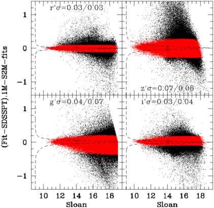
Fig. 23.— S2M fits with seven g′ r′ i′ z′ JHK2/s bands for ∼1 million SDSS-PT standards with 2MASS magnitudes, to g′ ∼ 19 mag, plotted as Fit-SDSSPT vs. SDSSPT magnitudes in separate panels for g′ r′ i′ z′. Black dots show all the rejected stars. The red bands through the middle show 91% of stars left after sigma clipping in g′ and >95% of stars left in r′ i′ z′. The dashed-line histograms show the number distribution of errors about the mean for all the stars. The annotated sigmas are to a limiting magnitude of 16 in each band for the full magnitude range.
Figure 24 shows the distribution of these stars as absolute magnitude against V - I color. The larger SDSS-PT sample shows a more heavily populated lower main sequence than for the southern Sloan standards.
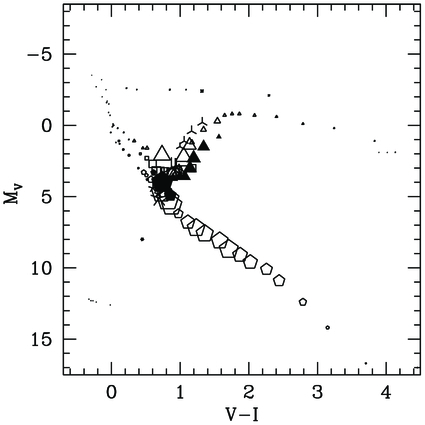
Fig. 24.— HR diagram for ∼1 million SDSS-PT standards. Symbols are as in Fig. 12.
Table 14 contains similar fitted data for 15,673 Sloan southern standards, where the name contains the original sexagesimal coordinates. Missing input magnitudes are listed as -9.999 with associated errors of +9.999.
8.3. Spectrally Matched Tycho2 Catalog
The catalog of 2.4 million fitted Tycho2 stars is listed in Table 15. For each star, it contains Tycho2 coordinates; proper motions in R.A./decl. in milliarcseconds yr-1; BT VT catalog magnitudes and errors; NOMAD Rn magnitudes; 2MASS J2 H2 K2/S magnitudes, mean errors, and quality flag; fitted values for rank; χ2; RTM (magnitude); number and type of matching spectrum; fitted BT VT; UBVRI - ZY magnitudes on the Vega system; fitted u′ g′ r′ i′ z′ magnitudes on the AB system; and distances in parsecs.
Because the Tycho2 catalog covers a wide range of optical magnitudes and colors, it also covers a wide range of 2MASS magnitudes. We have included bright 2MASS sources that have larger errors due to saturation effects: typically brighter than 5 mag in J, H, or KS.36 In these cases (about 40,000 entries with 2MASS quality flag C or D) the fits tend to be dominated by the optical, rather than the infrared, bands. About 11,000 entries lack mean error information (quality flag U); we assign 0.04, 0.05, and 0.06 mag mean errors for JHKS, respectively, to enable our spectral matching procedure to work with the quoted 2MASS upper magnitude limits. About 570 entries lack magnitude information (quality flag X) in one or more 2MASS bands; for these entries our catalog shows -9.999 mag, with an error of +9.999. This permits the matching process to proceed with negligible input from the affected band. The 2MASS quality flags are included in the electronic catalogs, and most entries are AAA.
The fitted optical and infrared magnitudes are compared with the catalog values in Figure 25, which illustrates the magnitude range in the optical (+2.4 to ∼15 mag) and infrared (-4.5 to ∼15 mag). A 3σ clip has been applied to all six bands, leaving 95%, 96%, 82%, 99%, 99%, and 99% of values in the BT VT, RN (matched to fitted Landolt R), and JHK2 bands, respectively. The resulting sigmas are 0.19, 0.11, 0.26, 0.03, 0.03, and 0.03 mag in BT VT RN JHK2, respectively, comparable with the quoted errors in these bands. The sigmas are 0.12 and 0.09 mag for BT VT to 13 and 12.5 mag, respectively. Our fitted BT VT magnitudes may be more accurate than the catalog values, as they are tied to the more accurate 2MASS photometry via the spectral matching process. Both rejected and included points are shown, as described in the figure. The fitted values for BT VT are listed in Table 15; other values can be derived by adding the library magnitude from Table 6 for the appropriate band and spectral type to the fitted V magnitude.
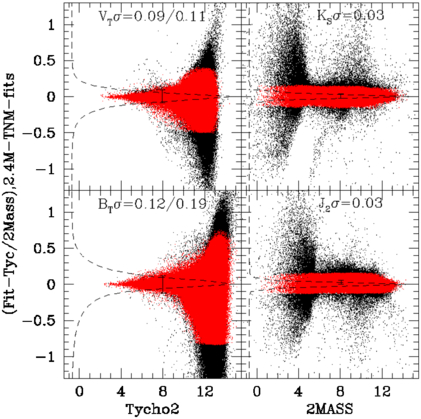
Fig. 25.— TNM fits with six BT VT RN J2 H2 K2 bands for ∼2.4 million Tycho2 stars with NOMAD RN and 2MASS JHK2 magnitudes, plotted as Fit-catalog vs. Tycho/2MASS catalog values on the abscissa. The Tycho2 catalog magnitudes vary between ∼2.4 and 16.5 mag. The 2MASS magnitudes reach as bright as −4.5 mag, but with significant errors there. Black dots show all the stars rejected by a 3σ clip to give the fitted dispersions shown. The red bands through the middle show 95%, 96%, 99%, and 99% of all stars left after sigma clipping in BT VT J2 K2, respectively. The dashed-line histograms, which show the number distributions of errors about the zero-delta line for all the stars, are quite strongly peaked around this line. The histograms are only slightly affected by the rejected points, as there are comparatively few of them. The annotated sigmas are to a limiting magnitude of 13 and 12.5 mag in BT VT and for the full magnitude range in each band.
Figure 26 shows the HR diagram derived for 2.4 million Tycho2 stars from these fits, which shows a less populated lower main sequence and a giant branch more dominated by solar metallicity stars than are the Landolt, SDSS-PT, or SDSS-southern standards, and about 3340 double-star DA1/K4V fits.
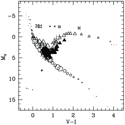
Fig. 26.— HR diagram for ∼2.4 million Tycho2 stars. Symbols are as in Fig. 12.
Figure 27 shows the same data plotted, where the size of the symbols now represents either the V light or the K light of the stellar types. The Tycho2 distribution is more dominated by solar-abundance types and by early giant branch types than is the SDSS-PT standard population.
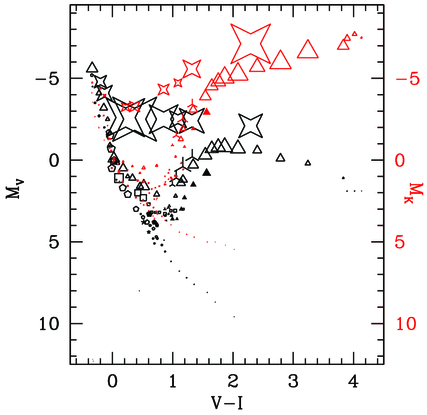
Fig. 27.— HR diagram for ∼2.4 million Tycho2 stars. The black symbols show the 141 library types plotted as MV vs. V - I, where the area of the symbols is proportional to the V light emitted by the stellar types. The red symbols occur on the same vertical line and are plotted as MK (on the right ordinate) vs. V - I, and the area of the symbols is proportional to the K light emitted by the stellar types. Symbols are as in Fig. 12.
8.4. Spectrally Matched Catalog of the SDSS Survey Region
The catalog of 4.8 million fitted Sloan survey stars with g < 16 is listed in Table 16, which contains the SDSS DR7 coordinates; unprimed ugriz (point-spread function [PSF]) magnitudes and errors for each star; matching 2MASS JHK2/S magnitudes, errors, and quality flag; fitted values of rank; χ2; Ruz, Rgz, and R2M; number and type of fitted spectrum; fitted UBVRI - ZY magnitudes on the Vega system; fitted u′ g′ r′ i′ z′ magnitudes; fitted (unprimed) ugriz magnitudes; and distances in parsecs. Other fitted magnitudes can be obtained by reference to Table 6.
The catalog contains about 100 entries with 2MASS quality flag X and about 43,000 entries with quality flag U, modified for magnitude and error, as detailed previously.
We found better fits to PSF magnitudes and errors than to model magnitudes and errors, so we have spectrally matched the PSF magnitudes. The difference between PSF and model magnitudes typically exceeds what would be expected from the DR7 quoted errors.
Figure 28 shows the comparison of DR7 griz magnitudes with our fitted unprimed griz magnitudes. There are quite a large number (about 30%) of discrepant points in one or more DR7 bands. In this case we have initially rejected points with large values of Rgz and then performed the sigma clip to reduce the numbers only slightly. The sigmas after this process are 0.18, 0.06, 0.04, 0.04, and 0.05 for ugriz, respectively, and (by reference to § 6.3.2) are inferred to be similar for UBVRI. For about 70% of the DR7 survey stars to g < 16, these S2M fits are reported as the typical 1σ error per DR7 star per band in the Abstract.
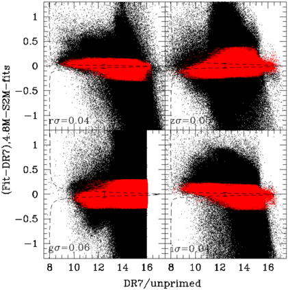
Fig. 28.— S2M fits with eight ugrizJHK2 bands for ∼4.8 million SDSS stars to g < 16 with unprimed ugriz and 2MASS JHK2 magnitudes, plotted as Fit-DR7 values on the ordinate and DR7 values on the abscissa. Black dots show all the stars rejected by an Rgz and 3σ clip to give the fitted dispersions shown. The red bands through the middle show about 70% of stars left after Rgz and sigma clipping, The dashed-line histograms show the number distributions of errors. They are reasonably well peaked about the zero-delta line, but there are a surprisingly large number of discrepant points at relatively bright magnitudes and near the zero-delta line.
There are quite a large number of (black) points rejected by the preceding process at relatively bright magnitudes and near the zero-delta line in each panel. This is because many of the ∼30% points rejected as having large Rgz values are seriously discrepant in one or more color bands, but fit well in other colors. It is possible, but not verifiable here, that transparency variations during the drift scans have affected different color bands for different stars. Unfortunately, the quoted PSF errors are often quite low when the magnitudes appear to be severely discrepant, so our fitting process has trouble discriminating between accurate and doubtful data.
Note that the number of rejected points per histogram bin away from the peak is only 1–3% of those at the peak, but summed over ∼20 such bins contain about 30% of the (rejected) data points. The histogram bin size was increased from 0.05 to 0.1 mag here to emphasize the outlying values.
The R2M values in Table 16 are based on the rms differences between the 2MASS catalog and fitted values. Their sigma-clipped values are 0.04, 0.05, and 0.06 mag for JHK2, respectively.
Figure 29 shows the HR diagram derived for 4.8 million SDSS stars to g < 16 from these fits, where the symbol area is proportional to the number of occurrences of each type.
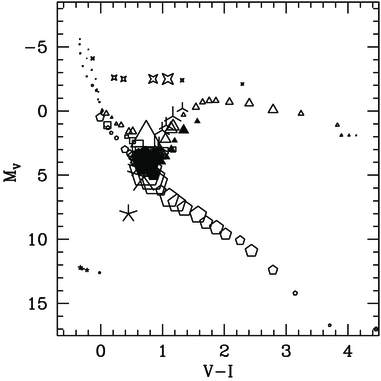
Fig. 29.— HR diagram for ∼4.8 million SDSS stars to g < 16. Symbols are as in Fig. 12, with symbol area proportional to number of occurrences.
Figure 30 shows the same data plotted as MV and MK vs. V - I, where the symbol area is proportional to the V light and K light, respectively.
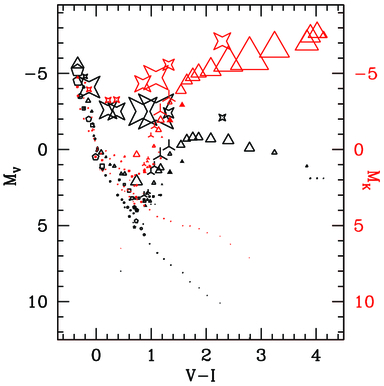
Fig. 30.— HR diagram for ∼4.8 million SDSS stars to g < 16 : Symbols are as in Fig. 12, with black symbols plotted as MV vs. V - I,red symbols plotted as MK vs. V - I, and symbol area proportional to the V light or K light emitted by the stellar types.
Our fitted magnitudes may improve over discrepant points in individual filter bands in the input catalog values, since the spectral matching process associates fitted values in each band with additional, sometimes more accurate, data.
9. SUMMARY
We present online catalogs that provide synthetically calibrated and fitted magnitudes in several standard filter system bandpasses for several surveys, including the all-sky Tycho2 survey and the Sloan survey region to g < 16. The errors of the synthesized magnitudes are mainly limited by the accuracy of the input data, but sufficient stars should be available in fields of view ≥30′ to average enough stars to provide flux calibrations to better than 10%, and often better than 5%, in most bandpasses and most observing conditions. For instance, with nine Tycho2 stars in a typical 30′ field of view, flux calibration to about 0.1, 0.05, 0.04, 0.03, and 0.03 mag should be possible in either UBVRI or u′ g′ r′ i′ z′ systems. These are typically achievable field-to-field uncertainties on either standard system. Relative calibration of repeated images of the same field, with similar or different equipment, should be automatically possible to 2% or better, even during variable photometric conditions, but subject to the preceding averaged systemic uncertainty.
The spectral matching technique provides a standard photometric system check on survey magnitudes and, because of matching to multiple filter bands, can be more accurate than individual measurements in some filter bandpasses. The accuracy of fitted magnitudes improves substantially with improving survey data accuracy, as does the reliability of fitted types, luminosity classes, and distances. The method enables quick statistical analyses of stellar populations sampled by wide-field surveys.
Substantial improvements can be expected in terms of reliable types, multifilter magnitudes, and distances with realistic improvements in the spectral library definition (e.g., the Next Generation Spectral Library [Gregg et al. 2006; Heap & Lindler 2010]) and expected all-sky survey improvements, but, importantly, only a few accurately determined survey bands (spanning optical and infrared bands) are typically necessary to derive accurate multifilter fits. Spectral matching removes the necessity to accurately measure all desired filter bandpasses in all-sky surveys.
We acknowledge the referee who suggested several useful improvements. We would like to acknowledge the extensive standard system photometry referenced here and the producers and maintainers of the CALSPEC database at Space Telescope Science Institute. This research has made extensive use of the Tycho2, 2MASS, SDSS DR7, and NOMAD catalogs, and we gratefully acknowledge their producers. We have made use of the SIMBAD database operated at Centers de Données, Strasbourg, France, and of several data access tools provided through the cdsclient package.
Online Material
Footnotes
- 1
- 2
- 3
- 4
- 5
- 6
- 7
- 8
- 9
21.0999 = -2.5 ∗ log 10(3631e-12 ergs·cm-2·s-1·A-1).
- 10
- 11
- 12
- 13
- 14
- 15
- 16
- 17
- 18
- 19
See http://lcogt.net.
- 20
- 21
- 22
- 23
- 24
- 25
- 26
- 27
- 28
- 29
- 30
- 31
- 32
- 33
- 34
- 35
- 36