How hierarchical navigable small world (HNSW) algorithms can improve search

Do you know Kevin Bacon? The six degrees of separation rule says that if you map the right social connections, all people are six or fewer handshakes away from each other—including Kevin Bacon.

This game demonstrates the principle that underlies navigable small worlds, half of the concept powering hierarchical navigable small worlds (HNSW), an approximate nearest neighbors (ANN) algorithm that supports highly scalable vector search.

Modern applications frequently deal with high-dimensional data that includes embeddings of images, text, and more. A k-Nearest Neighbors (KNN) search tends to be impractical in these settings because KNN scalability breaks down as dimensionality increases.

ANN algorithms are slightly less accurate but are much faster—a worthy tradeoff. If you want to build similarity or vector similarity search functions, recommendation engines, or AI apps, an ANN algorithm will be a better choice than KNN.

That said, not all ANN algorithms are created equal. Many ANN algorithms introduce latency issues, performance bottlenecks, and scalability issues—improving on KNN but not realizing the full potential necessary for many use cases.

In recent years, the HNSW approach has emerged as the leading choice for teams building apps and features that require high-performance ANN algorithms. But what is it, how does it work, and how does it perform?

What is a hierarchical navigable small world (HNSW)?

Hierarchical navigable small world, or HNSW, is a graph-based ANN algorithm that combines navigable small worlds (networks of points where each point is connected to its nearest neighbors) and hierarchy (layers that refine search to support speed). Researchers Yu A. Malkov and D. A. Yashunin introduced the idea in the 2016 paper, “Efficient and robust approximate nearest neighbor search using Hierarchical Navigable Small World graphs.”

Unlike other ANN algorithms, which tend to require an exhaustive and often slow search, HNSW provides a graph that minimizes hops from point to point and a hierarchy that doesn’t require many distance computations. The combination of the two is what makes HNSW stand apart from other ANN algorithms: One study found that, in comparison to other ANN algorithms, “Over all recall values, HNSW is fastest.”

HNSW algorithms also tend to outcompete ANN algorithms in practical terms. Many ANN methods require a training phase, but HNSW doesn’t, meaning teams can build the HNSW incrementally and update it over time.

Because of its performance and practicality, HNSW shines in numerous use cases, including:

• Image recognition and retrieval, where search functions have to search across high-dimensional vectors.
• Natural language processing (NLP), where it can support semantic and similarity search functions.
• Recommendation engines, where it can suggest a relevant product for a shopper or highlight the best paragraph from a help center to assist a user with troubleshooting.
• Anomaly detection, where it can support search across large datasets to detect fraud and monitor networks.

HNSW is growing in popularity because it’s better than most other ANN algorithms at supporting high-dimensional vector searches—a broad use case that’s only becoming more high-priority with the rise of AI.

How Does HNSW Work?

HNSW combines a hierarchy of layers with networks of navigable small worlds, allowing for scalable, high-performant search. Understanding HNSW requires understanding each half and how they come together.

The hierarchy comprises layers of data points, with the lowest layers containing all the data points and higher layers containing subsets of all the data points. The top layer is the sparsest, and the layers get denser with data the further down you go.

In contrast, other data point indexing methods are flat, meaning that the database stores the data points in their original form and without hierarchy. When you query across flat indexes, the algorithm has to scan each vector linearly, lending accuracy while enduring a computationally intense, slow process.

With a hierarchy, queries go from layer to layer, from top to bottom—resembling a skip list. In each layer, queries find a local minimum before dropping down a layer. This approach is probabilistic, meaning the search is much faster but slightly less accurate. As Malkov and Yashunin write in the original paper, “Starting search from the upper layer together with utilizing the scale separation boosts the performance compared to NSW and allows a logarithmic complexity scaling.”

Each layer uses a small world structure that graphs connections among data points. Each data point is linked to numerous neighbors, which ensures the average length of the path between any given data point and another is short. As you construct the HNSW index and select each layer a given vector goes into, the algorithm runs a “greedy search,” which finds the closest connections in each layer for the new vector. This is how HNSW maintains navigability and ensures each small world remains small.

Together, the hierarchy and the navigable small worlds enable efficient search. Queries can navigate the small worlds of each layer quickly and then rapidly sort through the data set layer by layer.

HNSW is even more effective when you use parameter tuning.

• M (the maximum number of connections per node) determines the number of neighbors a node can have in the graph. Higher M increases the indexing size and time. Lower M reduces memory usage and indexing time.
• efConstruction determines how thoroughly the graph will be searched as you insert new elements. High efConstruction results in better search accuracy—lower efConstruction results in faster indexing. 
• efSearch determines the size of the candidate list during search. Higher efSearch results in greater accuracy—lower efSearch results in faster queries.

Tuning these parameters is a game of trade-offs, allowing you to dial in your preferred amount of indexing time, memory usage, and accuracy.

HNSW is at its most effective when you use it for large datasets—especially ones that include over one million documents—and in situations when search performance and scalability are higher priorities than perfect accuracy.

How does HNSW compare to other ANN approaches?

There isn’t a one-size-fits-all choice for ANN indexing strategies, but when you compare HNSW to other approaches, HNSW tends to have some significant advantages.

HNSW vs. KD-Trees

KD-Trees (k-dimensional tree) is an approach to organizing data points in a multi-dimensional space. Like HNSW, the emphasis is on enabling you to search for nearby points quickly. With KD-Trees, the core structure is a decision tree for each space. At each level, the decision splits into halves and one dimension is chosen at a time. Queries traverse each tree to find candidate neighbors.

KD-Trees tend to work well for low-dimensional data, but search performance can degrade as dimensionality increases. HNSW, in contrast, can maintain search speed even when the data structure gets complex.

HNSW vs. Locality-Sensitive Hashing (LSH)

LSH is an approach to organizing data that uses random hash functions to bucket similar vectors so that searches can find the right ones quickly. By hashing the query, searches can only look up vectors in a corresponding bucket, meaning they don’t have to scan everything.

LSH tends to be best in cases where the data is extremely high-dimensional, or vectors are sparse. LSH is memory efficient, but recall can suffer as a result, which means HNSW is often a better approach for teams that need high accuracy, even if HNSW tends to require greater memory usage.

HNSW vs. Inverted File Index (IVF)

IVF is an indexing technique focused on clustering. With this approach, you partition the vector database into clusters before indexing and give each cluster a representative centroid. The index is split into inverted lists, each containing vectors assigned to that cluster. When you run queries, you only compare the query to vectors in a select few clusters instead of the whole set.

Overall, IVF tends to be one of the fastest options available, especially for large datasets, but it can suffer from below-average recall—especially when compared to approaches like HNSW. IVF also needs upfront clustering work, whereas HNSW can be iterated incrementally.

What are the tradeoffs and challenges with HNSW?

HNSW has advantages over many other approaches, but it’s not without its tradeoffs, and some use cases will benefit from other techniques.

High memory consumption

HNSW, due to its graph-based structure, requires much more memory than other ANN methods. With larger amounts of connections per node, HNSW can get even more memory-intensive. Tuning parameter M can help find a balance, and using lower-dimensional embeddings can make functions more efficient, but there still tends to be a practical limit on graph size.

Index construction overhead

HNSW, due to the hierarchy it requires, can be computationally expensive, and the queries run using it can be time-consuming. For every new point, HNSW performs a greedy search to find the best neighbors and updates the graph by inserting connections—a process that it has to repeat for every new point.

Tuning efConstruction, which controls the thoroughness of the search, can allow you to dial in the best balance of indexing time vs. accuracy. Similarly, using parallel index construction, which allows you to use multi-threading, can make the work less intensive. As a result, database products that offer parallelized index construction, incremental updates, and easily configurable efConstruction can be best for companies looking to reduce indexing time.

Scalability challenges

HNSW is best for in-memory, monolithic indexing, so it tends to suffer in distributed environments. HNSW is shardable, but sharding creates additional complexity and requires more memory to manage the various pieces.

Clustering solutions such as Redis clustering can, however, help distribute workloads. Starlogik, for example, uses a single Redis cluster to process 100 million calls per day and thousands of calls per second.

Trade-offs in accuracy vs. speed

Managing an HNSW implementation requires finding the right balance between accuracy and speed. Higher M lowers speed, for example, but lowering it reduces memory usage; higher efSearch increases search accuracy, as another example, but lowering efSearch results in faster indexing.

There will never be a balance that’s perfect for all contexts. Instead, finding the right balance will require looking closely at the use case at hand. Generally speaking, you can tune to the right balance by starting with the defaults, measuring recall and latency on a validation data set, increasing efSearch if recall is low, and increasing M and efConstruction if recall remains too low. Incremental tuning allows you to find the right level of recall without overburdening performance.

Database products that offer dynamic search tuning, optimized query execution, and adaptive indexing strategies can help you further balance recall and response times.

HNSW implementation best practices

HNSW poses significant advantages over many other ANN approaches, but those advantages only bear out when you implement it well. Following the below best practices will give you the best chance to see HNSW in its best light.

1. Optimize memory usage: Memory usage in HNSW is primarily caused by the number of graph connections and the amount of vector storage, so you can optimize memory usage by reducing edges (lowering M) or compressing vectors (FAISS, for example, supports this).
2. Tune your parameters to balance recall and speed: Different workloads will require different balances between efConstruction and M. Lowering M can reduce indexing time, for example, and increasing efConstruction can make search more accurate.
3. Use parallel index construction: Many HNSW implementations support multi-threading. Configure numerous threads to build simultaneously to construct indexes in parallel and significantly boost build times.
4. Use dynamic index updates to avoid full re-indexing: Rebuilding an entire HNSW index after every data change can be slow, wasteful, and disruptive. Instead, insert new vectors incrementally and delete old ones (or mark them inactive). Pruning old vectors and slowly adding new ones allows you to avoid the biggest speed issues.
5. Dimensionality reduction: Use random projection to reduce the number of dimensions in a vector by specifying the option and the number of dimensions.

With these best practices, you can turn HNSW—already a highly effective approach—into a truly scalable solution, even for distributed environments.

Redis supports scalable and high-performance HNSW search

HNSW is, overall, an effective approach to building scalable, accurate, and efficient search features, but HNSW works best with optimized vector database solutions. As a result, the best search features often come from combining the two.

Redis offers built-in support for HNSW-based ANN search, which simplifies implementation and enables teams to hit the ground running with both.

Redis 8, for example, can sustain 66K vector insertions per second for an indexing configuration that allows precision of at least 95% (M 16 and EF_CONSTRUCTION 32)—even at a billion-vectors scale while employing real-time indexing.

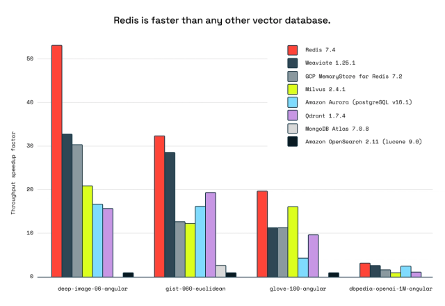
We’ve also benchmarked our performance against other vendors, with our testing showing that Redis is faster for vector database workloads than any other vector database we tested. Overall, Redis has 62% more throughput than the second-ranked database for lower-dimensional datasets and 21% more throughput for high-dimensional datasets.

Vector storage and rapid data retrieval are only becoming more sought after with the rise of generative AI. Redis helps companies handle AI workloads at scale, which OpenAI experienced working with Redis to scale ChatGPT. Redis “plays a crucial role in our research efforts,” according to a blog post from OpenAI. “Their significance cannot be understated—we would not have been able to scale ChatGPT without Redis.”

Since HNSW performs best when supporting high-performance vector search, Redis is an ideal product to work with if HNSW sounds like a good fit for your workloads. Redis offers, for example:

• Efficient, in-memory vector storage.
• Real-time speeds of search performance.
• Native support for clustering and scaling.

HNSW is at its best when you can finetune it to your precise use case and needs, which you can do manually, but Redis provides a pre-built, scalable version that’s easy to configure.

In the example below, running the code creates an index named documents over hashes with the key prefix docs and an HNSW vector field named doc_embedding with five index attributes: TYPE, DIM, DISTANCE_METRIC, M, and EF_CONSTRUCTION.

Ready to experience the speed and efficiency of Redis for HNSW-based ANN search? Try Redis now or schedule a demo to see how it can optimize your search performance.