#!/usr/bin/env python
# coding: utf-8
# <!--BOOK_INFORMATION-->
# <img align="left" style="padding-right:10px;" src="figures/PDSH-cover-small.png">
# *This notebook contains an excerpt from the [Python Data Science Handbook](http://shop.oreilly.com/product/0636920034919.do) by Jake VanderPlas; the content is available [on GitHub](https://github.com/jakevdp/PythonDataScienceHandbook).*
#
# *The text is released under the [CC-BY-NC-ND license](https://creativecommons.org/licenses/by-nc-nd/3.0/us/legalcode), and code is released under the [MIT license](https://opensource.org/licenses/MIT). If you find this content useful, please consider supporting the work by [buying the book](http://shop.oreilly.com/product/0636920034919.do)!*
#
# *No changes were made to the contents of this notebook from the original.*
# <!--NAVIGATION-->
# < [Aggregations: Min, Max, and Everything In Between](02.04-Computation-on-arrays-aggregates.ipynb) | [Contents](Index.ipynb) | [Comparisons, Masks, and Boolean Logic](02.06-Boolean-Arrays-and-Masks.ipynb) >
# # Computation on Arrays: Broadcasting
# We saw in the previous section how NumPy's universal functions can be used to *vectorize* operations and thereby remove slow Python loops.
# Another means of vectorizing operations is to use NumPy's *broadcasting* functionality.
# Broadcasting is simply a set of rules for applying binary ufuncs (e.g., addition, subtraction, multiplication, etc.) on arrays of different sizes.
# ## Introducing Broadcasting
#
# Recall that for arrays of the same size, binary operations are performed on an element-by-element basis:
# In[4]:
import numpy as np
# In[5]:
a = np.array([0, 1, 2])
b = np.array([5, 5, 5])
a + b
# Broadcasting allows these types of binary operations to be performed on arrays of different sizes–for example, we can just as easily add a scalar (think of it as a zero-dimensional array) to an array:
# In[6]:
a + 5
# We can think of this as an operation that stretches or duplicates the value ``5`` into the array ``[5, 5, 5]``, and adds the results.
# The advantage of NumPy's broadcasting is that this duplication of values does not actually take place, but it is a useful mental model as we think about broadcasting.
#
# We can similarly extend this to arrays of higher dimension. Observe the result when we add a one-dimensional array to a two-dimensional array:
# In[7]:
M = np.ones((3, 3))
M
# In[8]:
M + a
# Here the one-dimensional array ``a`` is stretched, or broadcast across the second dimension in order to match the shape of ``M``.
#
# While these examples are relatively easy to understand, more complicated cases can involve broadcasting of both arrays. Consider the following example:
# In[9]:
a = np.arange(3)
b = np.arange(3)[:, np.newaxis]
print(a)
print(b)
# In[10]:
a + b
# Just as before we stretched or broadcasted one value to match the shape of the other, here we've stretched *both* ``a`` and ``b`` to match a common shape, and the result is a two-dimensional array!
# The geometry of these examples is visualized in the following figure (Code to produce this plot can be found in the [appendix](06.00-Figure-Code.ipynb#Broadcasting), and is adapted from source published in the [astroML](http://astroml.org) documentation. Used by permission).
# 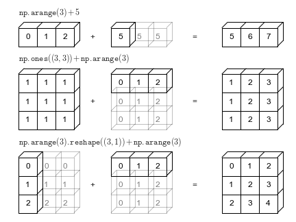
# The light boxes represent the broadcasted values: again, this extra memory is not actually allocated in the course of the operation, but it can be useful conceptually to imagine that it is.
# ## Rules of Broadcasting
#
# Broadcasting in NumPy follows a strict set of rules to determine the interaction between the two arrays:
#
# - Rule 1: If the two arrays differ in their number of dimensions, the shape of the one with fewer dimensions is **padded** with ones on its leading (left) side.
# - Rule 2: If the shape of the two arrays does not match in any dimension, the array with shape equal to 1 in that dimension is **stretched** to match the other shape.
# - Rule 3: If in any dimension the sizes disagree and neither is equal to 1, an error is raised.
#
# To make these rules clear, let's consider a few examples in detail.
# ### Broadcasting example 1
#
# Let's look at adding a two-dimensional array to a one-dimensional array:
# In[11]:
M = np.ones((2, 3))
a = np.arange(3)
# Let's consider an operation on these two arrays. The shape of the arrays are
#
# - ``M.shape = (2, 3)``
# - ``a.shape = (3,)``
#
# We see by rule 1 that the array ``a`` has fewer dimensions, so we pad it on the left with ones:
#
# - ``M.shape -> (2, 3)``
# - ``a.shape -> (1, 3)``
#
# By rule 2, we now see that the first dimension disagrees, so we stretch this dimension to match:
#
# - ``M.shape -> (2, 3)``
# - ``a.shape -> (2, 3)``
#
# The shapes match, and we see that the final shape will be ``(2, 3)``:
# In[12]:
M + a
# ### Broadcasting example 2
#
# Let's take a look at an example where both arrays need to be broadcast:
# In[13]:
a = np.arange(3).reshape((3, 1))
b = np.arange(3)
# Again, we'll start by writing out the shape of the arrays:
#
# - ``a.shape = (3, 1)``
# - ``b.shape = (3,)``
#
# Rule 1 says we must pad the shape of ``b`` with ones:
#
# - ``a.shape -> (3, 1)``
# - ``b.shape -> (1, 3)``
#
# And rule 2 tells us that we upgrade each of these ones to match the corresponding size of the other array:
#
# - ``a.shape -> (3, 3)``
# - ``b.shape -> (3, 3)``
#
# Because the result matches, these shapes are compatible. We can see this here:
# In[14]:
a + b
# ### Broadcasting example 3
#
# Now let's take a look at an example in which the two arrays are not compatible:
# In[15]:
M = np.ones((3, 2))
a = np.arange(3)
# This is just a slightly different situation than in the first example: the matrix ``M`` is transposed.
# How does this affect the calculation? The shape of the arrays are
#
# - ``M.shape = (3, 2)``
# - ``a.shape = (3,)``
#
# Again, rule 1 tells us that we must pad the shape of ``a`` with ones:
#
# - ``M.shape -> (3, 2)``
# - ``a.shape -> (1, 3)``
#
# By rule 2, the first dimension of ``a`` is stretched to match that of ``M``:
#
# - ``M.shape -> (3, 2)``
# - ``a.shape -> (3, 3)``
#
# Now we hit rule 3–the final shapes do not match, so these two arrays are incompatible, as we can observe by attempting this operation:
# In[16]:
M + a
# Note the potential confusion here: you could imagine making ``a`` and ``M`` compatible by, say, padding ``a``'s shape with ones on the right rather than the left.
# But this is not how the broadcasting rules work!
# That sort of flexibility might be useful in some cases, but it would lead to potential areas of ambiguity.
# If right-side padding is what you'd like, you can do this explicitly by reshaping the array (we'll use the ``np.newaxis`` keyword introduced in [The Basics of NumPy Arrays](02.02-The-Basics-Of-NumPy-Arrays.ipynb)):
# In[17]:
a[:, np.newaxis].shape
# In[18]:
M + a[:, np.newaxis]
# Also note that while we've been focusing on the ``+`` operator here, these broadcasting rules apply to *any* binary ``ufunc``.
# For example, here is the ``logaddexp(a, b)`` function, which computes ``log(exp(a) + exp(b))`` with more precision than the naive approach:
# In[19]:
np.logaddexp(M, a[:, np.newaxis])
# For more information on the many available universal functions, refer to [Computation on NumPy Arrays: Universal Functions](02.03-Computation-on-arrays-ufuncs.ipynb).
# ## Broadcasting in Practice
# Broadcasting operations form the core of many examples we'll see throughout this book.
# We'll now take a look at a couple simple examples of where they can be useful.
# ### Centering an array
# In the previous section, we saw that ufuncs allow a NumPy user to remove the need to explicitly write slow Python loops. Broadcasting extends this ability.
# One commonly seen example is when centering an array of data.
# Imagine you have an array of 10 observations, each of which consists of 3 values.
# Using the standard convention (see [Data Representation in Scikit-Learn](05.02-Introducing-Scikit-Learn.ipynb#Data-Representation-in-Scikit-Learn)), we'll store this in a $10 \times 3$ array:
# In[20]:
X = np.random.random((10, 3))
# We can compute the mean of each feature using the ``mean`` aggregate across the first dimension:
# In[21]:
Xmean = X.mean(0)
Xmean
# And now we can center the ``X`` array by subtracting the mean (this is a broadcasting operation):
# In[22]:
X_centered = X - Xmean
# To double-check that we've done this correctly, we can check that the centered array has near zero mean:
# In[23]:
X_centered.mean(0)
# To within machine precision, the mean is now zero.
# ### Plotting a two-dimensional function
# One place that broadcasting is very useful is in displaying images based on two-dimensional functions.
# If we want to define a function $z = f(x, y)$, broadcasting can be used to compute the function across the grid:
# In[24]:
# x and y have 50 steps from 0 to 5
x = np.linspace(0, 5, 50)
y = np.linspace(0, 5, 50)[:, np.newaxis]
z = np.sin(x) ** 10 + np.cos(10 + y * x) * np.cos(x)
# We'll use Matplotlib to plot this two-dimensional array (these tools will be discussed in full in [Density and Contour Plots](04.04-Density-and-Contour-Plots.ipynb)):
# In[25]:
get_ipython().run_line_magic('matplotlib', 'inline')
import matplotlib.pyplot as plt
# In[26]:
plt.imshow(z, origin='lower', extent=[0, 5, 0, 5],
cmap='viridis')
plt.colorbar();
# The result is a compelling visualization of the two-dimensional function.
# <!--NAVIGATION-->
# < [Aggregations: Min, Max, and Everything In Between](02.04-Computation-on-arrays-aggregates.ipynb) | [Contents](Index.ipynb) | [Comparisons, Masks, and Boolean Logic](02.06-Boolean-Arrays-and-Masks.ipynb) >